A transformation in linear algebra can be likened to functions in the sense that they both take an input and produce an output
In the context of linear algebra, both the input and output are vectors
To understand the transformation as a whole, we shall consider how every possible input vectors migrate to the corresponding output vector
Since all possible input vectors span the whole space, observing how they transform is equivalent to understanding the transformation of the entire space itself
Arbitrary transformation can get very complicated and hard to predict, so we will only limit ourselves to linear transformations
For now, we can intuitively understand a linear transformation as one that satisfies two key properties
All straight lines must remain straight lines after the transformation
The origin must remain fixed or unchanged under the transformation
The formal definition of linearity will be presented in later chapters
Just like functions, we can describe a linear transform numerically
VinputtransformationVoutput
Our objective is to find a mathematical representation that can take any appropriate vector as input and produce the corresponding output
The complexity of our problem is greatly reduced when we realize we can track the transformation as a whole by observing how it affects a set of basis vectors
Recall that any vector can be represented as a linear combination of the basis vectors
Upon transformation, all vectors, including the basis vectors, undergo the same degree of distortion. Consequently, any output vector can be obtained by applying the same linear combination to the transformed basis vectors
Numerically, this implies that the components of each transformed basis vector are equivalent to the components of the original basis vector
Hence, the action of a linear transformation is fully specified by its action on the basis vectors. If the basis vectors suffer a change, then any vector in this space will also undergo a change that is readily calculable
The ability to summarize a linear transformation using basis vectors is crucial
The derived expression reveals that the transformation of any vector can be computed once we know its components in the original basis and how the basis vectors are transformed
The components of the vector ( v1,v2,v3,⋯ ) comes from the input vector, which implies that the transformed basis vectors alone can describe the entire transformation
an array containing all necessary information[transformedbasis 1transformedbasis 2transformedbasis 3⋯]
By assembling all the transformed basis vectors together, this array encompasses all the information required to describe the linear transformation. We refer to this array as a matrix.
A matrix can be regarded as a collection of the transformed basis vectors, containing all the necessary information to perform a linear transformation
In this sense, a matrix functions as the operator for linear transformations
Similar to functions, we can find the output by applying the matrix to the input vector
matrix acting on input vector[transformedbasis 1transformedbasis 2transformedbasis 3⋯]Vinput=Voutput
To facilitate this computation, we express the input vector as a column vector
We have arrived at an expression for a matrix acting on an input vector. This operation, where a matrix acts on a vector, is commonly referred to as matrix-vector multiplication
To perform matrix-vector multiplication, it is necessary to have knowledge of the transformed basis vectors in terms of the original basis
We represent the transformed basis vectors as follows
By convention, the inner brackets within the matrix are often omitted. Performing vector addition, we arrive at a more general and commonly used expression for matrix-vector multiplication
So a linear transformation between dimension is just one that changes the number of entries of the input vector
When performing a linear transformation, the dimension of the input and output vectors is determined by the number of columns and rows of the transformation matrix, respectively
Each column of the matrix represents the coordinates of the transformed basis vector, which corresponds to the dimension of the input vector
Each row of the matrix represents a dimension of the transformed basis vectors, which corresponds to the dimension of the output vector
We can therefore determine how the dimension of the vector will change upon the transformation
If the number of columns is greater than the number of rows of the matrix, then the dimension of the vector will decrease upon transformation
If the number of columns is smaller than the number of rows of the matrix, then the dimension of the vector will increase upon transformation
If the number of columns and the rows of the matrix is the same, then the dimension of the vector remains unchanged. We call these type of matrices as square matrix
Linear transformation across dimensions give restrictions to when matrix-vector multiplication is possible
The dimension of the input vectors should be equal to the number of basis vectors needed to describe it
Hence, a matrix must contain the same number of basis vectors, which is given by the number of its columns, to fully describe the transformation of the input vector
Matrix-vector multiplication is therefore only possible when the number of column of the matrix mathces the dimension of the input vector
Since matrices can come in different shape and sizes, we have a convention that describes its dimension
m rowsn columns⎩⎪⎪⎪⎪⎪⎨⎪⎪⎪⎪⎪⎧⎣⎢⎢⎢⎢⎢⎡Ω11Ω21Ω31:Ωm1Ω12Ω22Ω32:Ωm2Ω13Ω23Ω33:Ωm3⋯⋯⋯⋯Ω1nΩ2nΩ3n:amn⎦⎥⎥⎥⎥⎥⎤
In many situations, we encounter the need to perform a series of successive linear transformations
The fundamental principle remains constant: the final transformation can be determined by tracking the set of basis vectors
The traditional approach to compute the final position of a vector involves multiplying the vector by the corresponding matrices one by one, in a nested fashion
However, this method can become tedious and cumbersome, especially when dealing with numerous transformation steps
A more efficient approach is to find the overall effect of the successive transformations
The matrix responsible for directly transforming the input vector to the final position is known as the composite matrix
[Composite Matrix]Vinput=Voutput
Since multiplying the vector by the composite matrix has the same effect as multiplying it by a series of individual matrices, we can establish the following equality
An interesting aspect to note is that matrix multiplication is performed from right to left in this context, which is analogous to the notation used for composite functions
To understand matrix multiplication, let's delve into the transformation of basis vectors in each step
second transformation⎣⎢⎢⎢⎡B11B21B31:B12B22B32:B13B23B33:⋯⋯⋯⎦⎥⎥⎥⎤first transformation⎣⎢⎢⎢⎡A11A21A31:A12A22A32:A13A23A33:⋯⋯⋯⎦⎥⎥⎥⎤=overall transformation⎣⎢⎢⎢⎡C11C21C31:C12C22C32:C13C23C33:⋯⋯⋯⎦⎥⎥⎥⎤
Recall that the columns of a matrix represent the transformed basis vectors. Therefore, the columns of the composite matrix represent the final transformed basis vectors
Not all matrix multiplications are allowed due to certain restrictions imposed by the dimensions of the matrices involved
Matrix multiplication is essentially composed of matrix-vector multiplications, so the restrictions imposed on matrix-vector multiplication translates to matrix multiplication as well.
Matrix-vector multiplication is only possible when the number of column of the matrix mathces the dimension of the input vector
The dimension of the each basis vector within the matrix is given by the number of rows of the matrix
Hence, matrix multiplication is only possible when the number of columns of the matrix on the left is equal to the number of rows of the matrix on the right
We can predict the dimension of a composite matrix simply by examining the dimension of the matrice that are being multiplied
The composite matrix should have the same number of columns as the dimension of the input vector and the dimension of the output vector is given by the number of rows
The matrix on the right is the one that takes the input and the matrix on the left governs the final dimension of the output vector
The composite matrix should therefore have the same number of columns as the matrix on the right and the same number of rows as the matrix on the left
We can assess whether a matrix multiplication is allowed and predict the dimension of the composite multiplication with a menmonic device
Brow×BcolumnMatrix B×Arow×AcolumnMatrix A
If Bcolumn=Arow, then the matrix multiplication is allowed
Given that the matrix multiplication is allowed, the composite matrix will have a dimension of Brow×Acolumn
Linear transformations are mathematical operations that can change vectors. However, they also have an impact on the space in which these vectors exist
In order to understand how the space changes during a linear transformation, we need a parameter that quantifies the distortion or warping of the space
One commonly used and intuitive parameter is the scaling factor of the n-dimensional space on which the transformation is applied. This scaling factor represents how much the space expands or contracts in different directions
To determine the scaling factor of space caused by a linear transformation, we introduce a function called the determinant
The argument of this function is a matrix that characterizes the linear transformation
The output of the function is the scaling factor accompanied by the transformation, which is just a scalar
The scaling factor of space encompasses two important aspects: magnitude and sign, which provide insights into changes in both the size and orientation of space resulting from a linear transformation
The magnitude of the scaling factor indicates the change in the size of space. Specifically, it represents the ratio between the original volume of the space and the volume of the transformed space
The sign of the scaling factor reflects changes in the orientation of space. Altering the orientation of space is akin to transforming it into its mirror image. Regardless of the dimension of the space, there are only two possible configurations for the orientation: a positive orientation and a negative orientation. Transformations that result in mirror images have a negative scaling factor, while transformations that preserve the orientation have a positive scaling factor
Determinants are only defined for linear transformations that do not result in a change in dimension
This is because the scaling factor of orientation and volume of space across dimension does not mean anything
Hence, only linear transformations that are characterized by square matrices can have a corresponding determinant
The determinant can be represented in two primary notations, each emphasizing the square matrix of the linear transformation we are studying
The first notation is a functional representation, where the determinant is denoted as a function with the square matrix as its argument
The second notation is an array representation, where the determinant is denoted using vertical bars, with the entries being the same as those in the square matrix
A practical approach to calculating the determinant involves viewing space through the concept of grid lines
A fundamental property of linear transformations is that the grids formed by the basis vectors must remain uniformly spaced and identical after the transformation
Consequently, the scaling factor of space is equivalent to the scaling factor of each individual grid. This observation stems from the fact that every part of space is identical and, therefore, experiences the same scaling factor
The size and orientation of these grids are conventionally defined by the chosen basis of the space. Hence, to calculate the determinant, we can examine how the basis vectors transform.
The grid formed by the n basis vectors represents an n-dimensional parallelotope
The volume of the n-dimensional parallelotope, in an oriented sense, provides the scaling factor, which is determined by the ratio of the oriented n-dimensional volume of the transformed parallelotope to the oriented n-dimensional volume of the original parallelotope
Scaling Factor=oriented n-dimensional volume of the original parallelotopeoriented n-dimensional volume of the transformed parallelotope
Since the original basis vectors are defined to have unit lengths and are properly oriented in their own basis, the denominator of the above expression simplifies to 1
Scaling Factor=1oriented n-dimensional volume of the transformed parallelotope
Hence, the determinant is given by the oriented n-dimensional volume of the parallelotope defined by the transformed basis vectors
To establish an expression for computing the determinant, it is essential to grasp the nature of the determinant and its inherent properties
Having defined the determinant to be a signed volume of the parallelotope formed by the basis vectors, several fundamental properties arise
We can select a few of these properties to define the determinant in terms of them.
Scaling of a Column and Determinant
When all the entries in a column of a matrix are scaled by a constant, the corresponding determinant is also scaled by the same constant
Since each column in the matrix corresponds to a basis vector, scaling all the entries of a column is equivalent to scaling the corresponding basis vector
Scaling the basis vector is equivalent to scaling one side of the parallelotope formed by the basis vectors, resulting in the volume of the parallelotope being scaled by the same amount
The determinant represents the volume of the parallelotope, so scaling the entries of a column also scales the determinant itself
When all entries in a column of a matrix can be expressed as the sum of two entries, the corresponding determinant can be separated into two determinants
Columns of a matrix represent basis vectors, and expressing all entries of a column as a sum corresponds to expressing the corresponding basis vector as a sum of two vectors
The volume obtained when adding a vector to another vector is equal to the sum of the volumes of the two vectors taken separately
The determinant gives us the volume of the parallelotope, so we can separate the determinant into two, where the only different column is the column of interest
The determinant remains unchanged even when subjected to a shearing transformation
Shearing represents a linear transformation that displaces every point in a fixed direction
Shearing can be achieved by adding a vector in the direction of one of the basis vectors that defines the parallelotope to another basis vector within the matrix
Shearing does not change the height of the parallelotope. Hence, the determinant, which represents the n-dimensional volume, is invariant under shearing
When two columns of a matrix are proportional to each other, the determinant becomes zero
Linearly dependent vectors cannot span the n-dimensional space, implying that their associated parallelotope's n-dimensional volume is zero
Consequently, when the set of basis vectors represented by the columns of a matrix is linearly dependent, the determinant evaluates to zero
This fundamental property allows the determinant to "detect" the linear dependency within a set of vectors
Determinant of Matrix Product
The determinant of the product of two matrices is equal to the product of their determinants
det(A^)×det(B^)=det(A^×B^)
The product of the determinants on the left-hand side of the equation represents the individual scaling factors of the transformations represented by matrices. Multiplying these scaling factors gives the scaling factor of the overall transformation
On the right-hand side, the determinant of the matrix product directly computes the scaling factor of the composed transformation
Antisymmetry of Determinants
Determinants exhibit an interesting property known as antisymmetry, which relates to the mirror image transformation of the parallelotope defined by the basis vectors
The relative positions of the basis vectors that define the n-dimensional parallelotope determine whether a transformation converts it into its mirror image
Whenever two basis vectors in the determinant are interchanged, the resulting parallelotope undergoes a mirror image transformation
Consequently, when two columns of a determinant are interchanged, the value of the determinant is multiplied by -1
Using the sum property of determinants, we can split the determinant into n new determinants. This fragmentation represents the subdivision of the n-dimensional volume into n parts
Although we are able to express the total volume of the parallelotope as a sum of other parallelotopes, we have yet taken orientations into account
Half of these fragmented parallelotope are in the positive space, while the other half are in the negative space and we cannot add parallelotopes that are inhabiting in different space together
In order ot perform the addition, we must ensure each of the fragmented parallelotope are back in the positive space by rearranging each of their orientations. We do so by putting the normalized vector back to the corresponding column
The antisymmetric property of determinants states that interchanging any two rows results in a change of sign. Hence, the sign of the determinant is negative for an odd number of row interchanges and positive for an even number of interchanges
Our rearrangement causes the sign of these fragmented determinants to have an alternating pattern of positive and negative signs
The simplification of the determinant not only simplifies the expression but also provides insights into the geometry of the problem
By analyzing the determinant expression, we can observe that each fragmented determinant can be split into two parts: a group of vectors that all lack a component in one of the basis directions, and a normalized vector that only has a component in that specific basis direction
The group of vectors lacking a component in one of the basis directions forms a parallelotope of dimension (n–1), while the remaining normalized vector is orthogonal to said parallelotope
Our determinant can be found if we can compute each of the fragmented n-dimensional volume and add all them up together
By multiplying the (n−1)-dimensional volume of the (n−1)-dimensional parallelotope with the height of the n-dimensional parallelotope, we obtain the n-dimensional volume of a n-dimensional parallelotope
The height, by definition, must be orthogonal to the (n−1)-dimensional parallelotope. In our context, the length of the normalized vector represents this height. Therefore, we can simplify the expression to
Since we are not concerned with units in this context, we can conclude that each fragmented n-dimensional parallelotope's volume has the same magnitude as its corresponding (n−1)-dimensional parallelotope
n-dimensional volume=(n – 1)-dimensional volume
This equivalence between the n-dimensional volume and the (n−1)-dimensional volume means that we can express the fragmented determinants of order n in terms of determinants of order (n−1)
We have successfully defined an expression for the determinant, allowing us to express an n-dimensional determinant in terms of (n−1)-dimensional determinants
This recursive definition might initially seem like an endless loop, but it is not the case as the dimension of the determinants is decreasing
Starting from an n-dimensional determinant, we can express it in terms of (n−1)-dimensional determinants, which can further be expressed in terms of (n−2)-dimensional determinants, and so on, until we eventually reach the 1-dimensional determinants
No matter where we start, we can always express our determinant in terms of some 1-dimensional determinants
As long as the 1-dimensional determinants are well defined, we can be confident that any n-dimensional determinants will also be well defined
An n-dimensional determinant represents the oriented n-dimensional volume. In the case of a 1-dimensional determinant, the oriented 1-dimensional signed-volume is simply the oriented-length of the vector.
Since a 1-dimensional determinant consists of a single one-dimensional vector, it has only one entry
This entry represents the oriented-length of the one-dimensional vector. Therefore, the output of a 1-dimensional determinant is equal to its entry
det([Ωij])=Ωij
By establishing this base case for 1-dimensional determinants, we can build upon it and recursively compute determinants of higher dimensions, allowing us to capture the oriented volumes of higher-dimensional parallelotopes
Having derived a general expression for determinants of any dimension, we can now introduce a mnemonic device that provides a practical method for computing determinants easily
We can take inspiration from our recurrence definition and express any determinant via the something called the Laplace Expansion
The Laplace expansion is a technique that allows us to express any determinant in terms of smaller determinants by systematically expanding along rows or columns
While the Laplace expansion is equivalent to the formula we derived earlier, it simplifies the computation process
We shall first define the minor for each entry
The minor ∣Mij∣ of entry Ωij of a determinant is the determinant obtained by deleting the ith row and jth column of the original determinant
The minors of a determinant of order n are determinants of order (n−1)
Every element in a determinant has a minor and their values are independent from each other
Furthermore, we assign a sign ( ± ) to each element based on its position within the determinant
The formula of the sign of each element is given by
(−1)i+j
The sign is positive when the sum of i and j is even and negative when it is odd
If we create an array of these signs, we will get an alternating pattern
⎣⎢⎢⎢⎡+−+:−+−:+−+:⋯⋯⋯⎦⎥⎥⎥⎤
Using the minors and the sign pattern, we can define the cofactor for each entry
The cofactor ∣Cij∣ of element aij is the product of the minor ∣Mij∣ and the appropriate sign of the element
∣Cij∣=(−1)i+j∣Mij∣
The cofactor shares the same magnitude as its corresponding minor but may have a different sign
The cofactor, just like the minor, is a determinant
For determinants of order greater than 1, we can expand them in terms of their elements using the cofactors
The general formula for the determinant is as follows
det(Ω^)=i=1∑nΩij∣Cij∣
This formula allows us to compute the determinant by summing the products of each element and its corresponding cofactor along any row or column
The specific row or column chosen does not affect the numerical value
Since each cofactor is itself a determinant, we can continue expanding it until we reach determinants of order 1, which are simply the individual elements of the original determinant
The effect of a linear transformation can be reversed by applying another transformation, which is known as the inverse transformation
Similarly, for matrices representing linear transformations, there exists a corresponding matrix that reverses the effect of the original matrix. This matrix is called the inverse matrix
We denote the inverse of a matrix with a superscript of −1
To establish an expression for computing the inverse of matrices, it is crucial to gain an understanding of their fundamental properties
By defining the inverse of a matrix as one that undoes its transformation, several immediate properties naturally emerge
Cancellation Property
Since the transformation caused by the inverse matrix cancels the effect of the original matrix, their composite matrix will have the effect of doing nothing
Ω^−1Ω^=Matrix That Does Nothing
A matrix that performs no transformation have its columns as the original basis vectors. We refer to this matrix as the identity matrix, I^
The definition of the inverse matrix can therefore be summarized as
A^−1Ω^=I^
The Identity Matrix
Multiplying any matrix by the identity matrix gives back the same matrix
Ω^I^=I^Ω^=Ω^
This is because the identity matrix does not perform any transformation, so the overall effect is just the other matrix
The Inverse of Composite Matrix
The inverse of a composite matrix is the product of the inverse matrices in reverse order
(A^B^)−1=(B^−1A^−1)
Reversing the order of the inverse matrices corresponds to reversing the effect of the transformations
-We can rationalize this as reversing the effect of linear transform from the last transformation to the first
The Inverse of an Inverse
The inverse of an inverse matrix is the original matrix
(Ω^−1)−1=Ω^
Just like how the inverse matrix cancels the effect of the original matrix, we can also say that the original matrix cancels the effect of the inversed matrix
Order of Multiplication
The order of multiplication between a matrix and its inverse does not affect the result
Ω^Ω^−1=Ω^−1Ω^=I^
This is because the inverse of an inverse matrix is the original matrix
Square Matrices and Inverses
Only square matrices have inverses
We have shown that Ω^Ω^−1 and Ω^−1Ω^ are both valid matrix-multiplication, which is only possible when
Ω^column=Ω^row−1andΩ^column−1=Ω^row
Moreover, both Ω^Ω^−1 and Ω^−1Ω^ produce the same matrix, I^, which means the dimension of the two composite matrices are the same
Ω^row=Ω^row−1andΩ^column=Ω^column−1
This means that Ωrow=Ωcolumn=Ωrow−1=Ωcolumn−1
In other words, only square matrices can have inverses
Determinant and Inverses
Only square matrices with a non-zero determinant are eligible to have inverses, while those with a determinant of zero do not
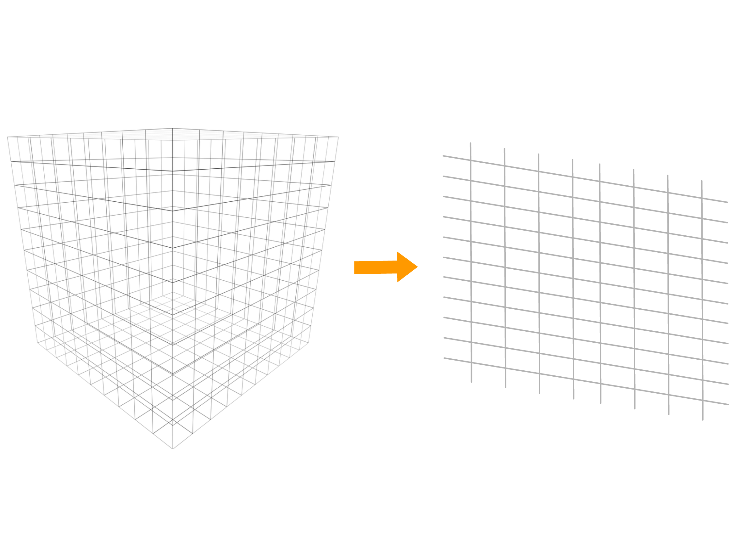
When the determinant of a square matrix is zero, the associated transformation compresses the space into a smaller dimension
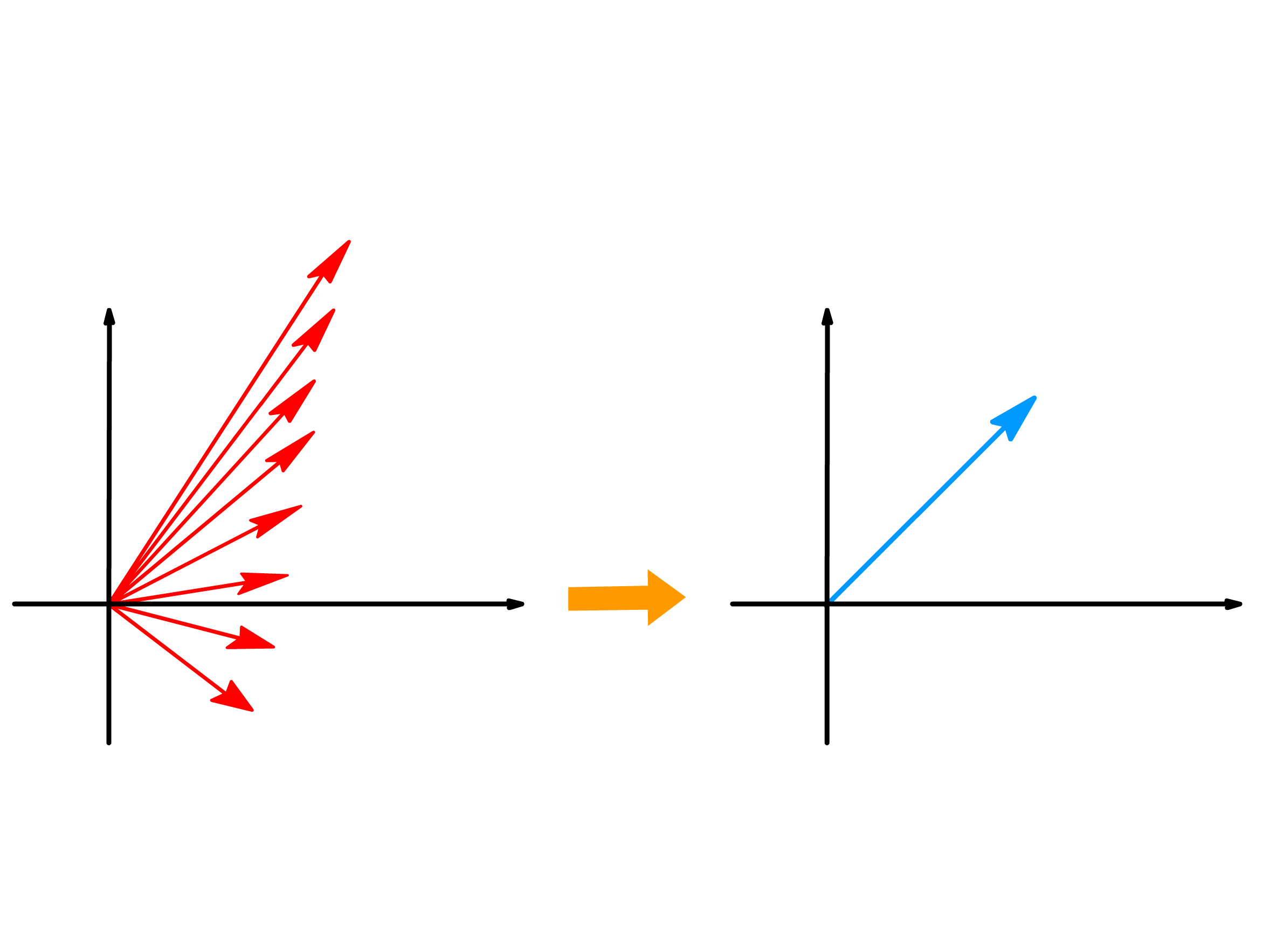
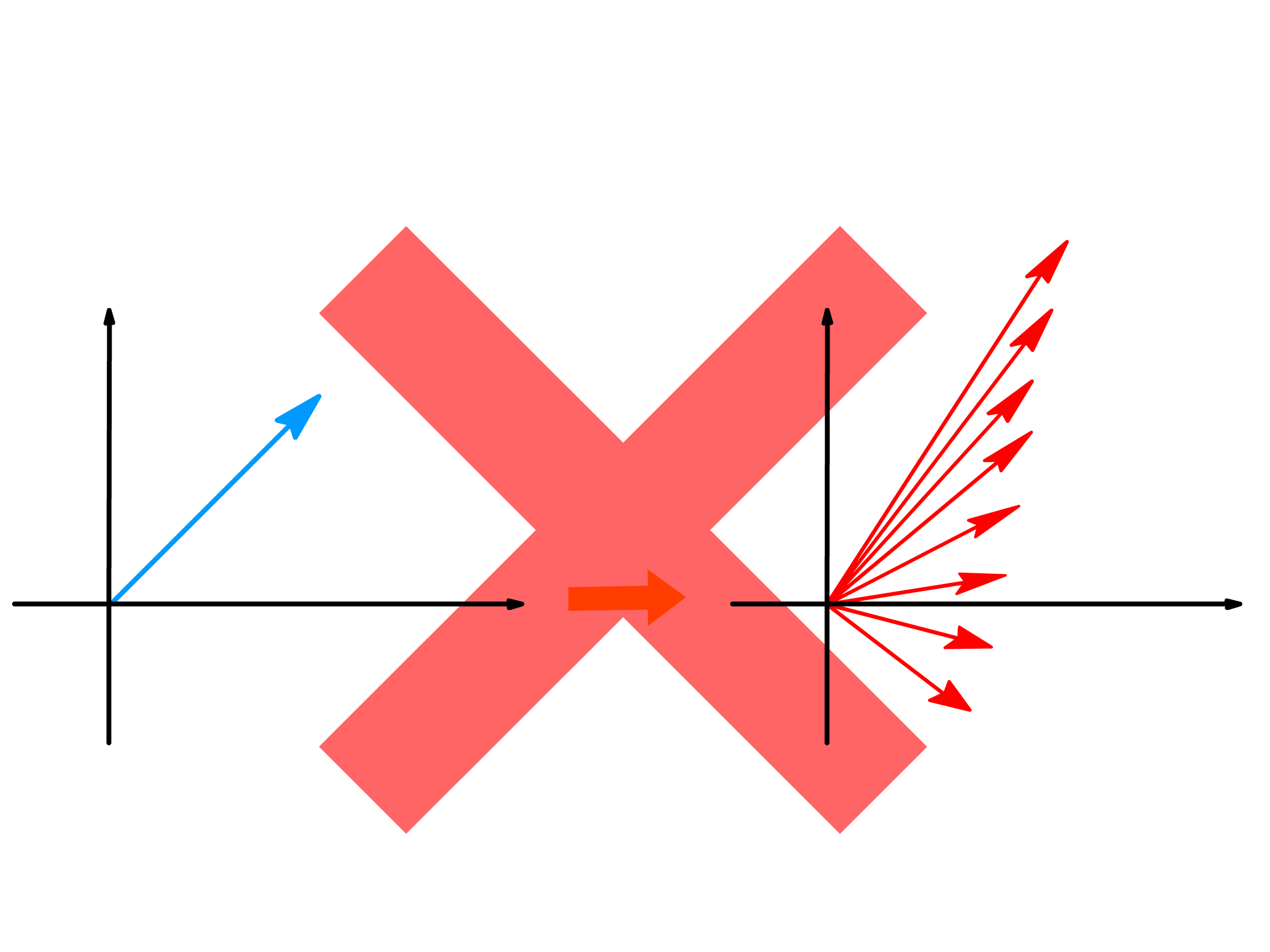
In these cases, the transformation collapses multiple distinct input vectors into the same output vector
To reverse such a transformation, an inverse matrix would need to produce multiple output vectors for a single input vector. However, allowing multiple output vectors violates the fundamental properties of linear transformations, rendering these types of transformations ineligible for inverses
To compute the inverse matrix, we can derive a general expression that allows us to determine each entry of the inverse
The inverse matrix is closely connected to the determinant, as both are defined only for square matrices, and the inverse exists only when the corresponding square matrix has a non-zero determinant
Therefore, we would expect the formula for the inverse matrix to involve the determinant
The goal of the derivation is to find a formula that allows us to determine each entry in the inverse matrix
Square matrices preserves the dimension of the input vectors, so they transform the input vectors by either scaling or rotating them, or a combination of both
Different input vectors will undergo unique scaling and rotation transformations
Linear transformations satisfy linearity, meaning that input vectors lying on the same line will also be transformed into output vectors lying on the same line
Some vectors in these transformations will only experience scaling without rotation, remaining on their original line after the transformation
These vectors, called eigenvectors, have associated eigenvalues, representing the scaling factor by which they stretch or compress during the transformation
Any vectors lying on the same line as an eigenvector are also eigenvectors, and they share the same eigenvalue
The concept of eigenvectors and eigenvalues can be expressed using a matrix-vector multiplication notation
Ω^eigen=(eigenvalue)eigen
This equation demonstrates that when a matrix acts on its eigenvector, the result is a scaling of said eigenvector by the corresponding eigenvalue
On the surface, the equation we just set up is a bit tricky to work with because it is equating a linear transformation with a scalar multiplication
To make our lives easier, we can write down the scalar multiplication in terms of a linear transformation. The definition of scalar multiplicaion is to scale all the basis vectors by the same amount, so the corresponding matrix will be
Having simplified our original equation, we can now attempt to solve it
There are only two possiblities, the eigenvector has no length and direction or the transformation squishes space into a smaller dimension. The latter gives us useful information, so we will focus on that
Option 1 :the eigenvector is a null vectoreigen=⎣⎢⎢⎢⎡000:⎦⎥⎥⎥⎤orOption 2 :squishes space into a lower dimension⎣⎢⎢⎢⎡Ω11−(eigenvalue)Ω21Ω31:Ω12Ω22−(eigenvalue)Ω32:Ω13Ω23Ω33−(eigenvalue):⋯⋯⋯⎦⎥⎥⎥⎤
Matrices associated with these kind of transformations must have a determinant of 0
Solving the system of equations will allow us to determine the ratios of the ♣i, but not their absolute values. This is related to the fact that vectors lying on the same line as an eigenvector are also eigenvectors with the same eigenvalues