¶ Macroscopic Description of Fluid Interfaces
¶ Surface Excess
Some solutes may not be uniformly distributed throughout a solution, as they can either accumulate at or avoid the interface
- In order to discuss this phenomenon in a quantitative manner, the concept of surface excess is introduced
Surface excess is a quantitative measure of the amount of a substance that accumulates at the interface, in excess of what would be expected based on its bulk concentration
- For a solute that accumulates at the surface, the surface excess is positive
- For a solute that avoids the surface, the surface excess is negative
We can write something similar for Gibbs energy as well
- Since the surface has no volume, we can express the differential of the surface Gibbs Energy as such at constant temperature
- The Euler's theorem allow us to write down , so its total differential is
- Equating both expressions of gives us the Gibbs-Duhem equation
- We shall define the surface excess per unit area as , the surface concentration
This equation can be interpreted as follows
- If adding more of solute (raising its chemical potential) decreases the surface tension, then is positive and solute will accumulate at the interface
- If adding more of solute (raising its chemical potential) increases the surface tension, then is negative and solute will avoid the interface
Similarly, we can express for a solute as a rate of change of surface tension with respect to its chemical potential
- We also refer to as the excess adsorption of a solute
¶ Dividing Surface
The interface between two phase is usually not a surface with zero thickness, in the sense that the surface is composed of one layer of molecules from each phases only
- The density profile is a measure of the distribution of molecules across the interfacial layer between two phases
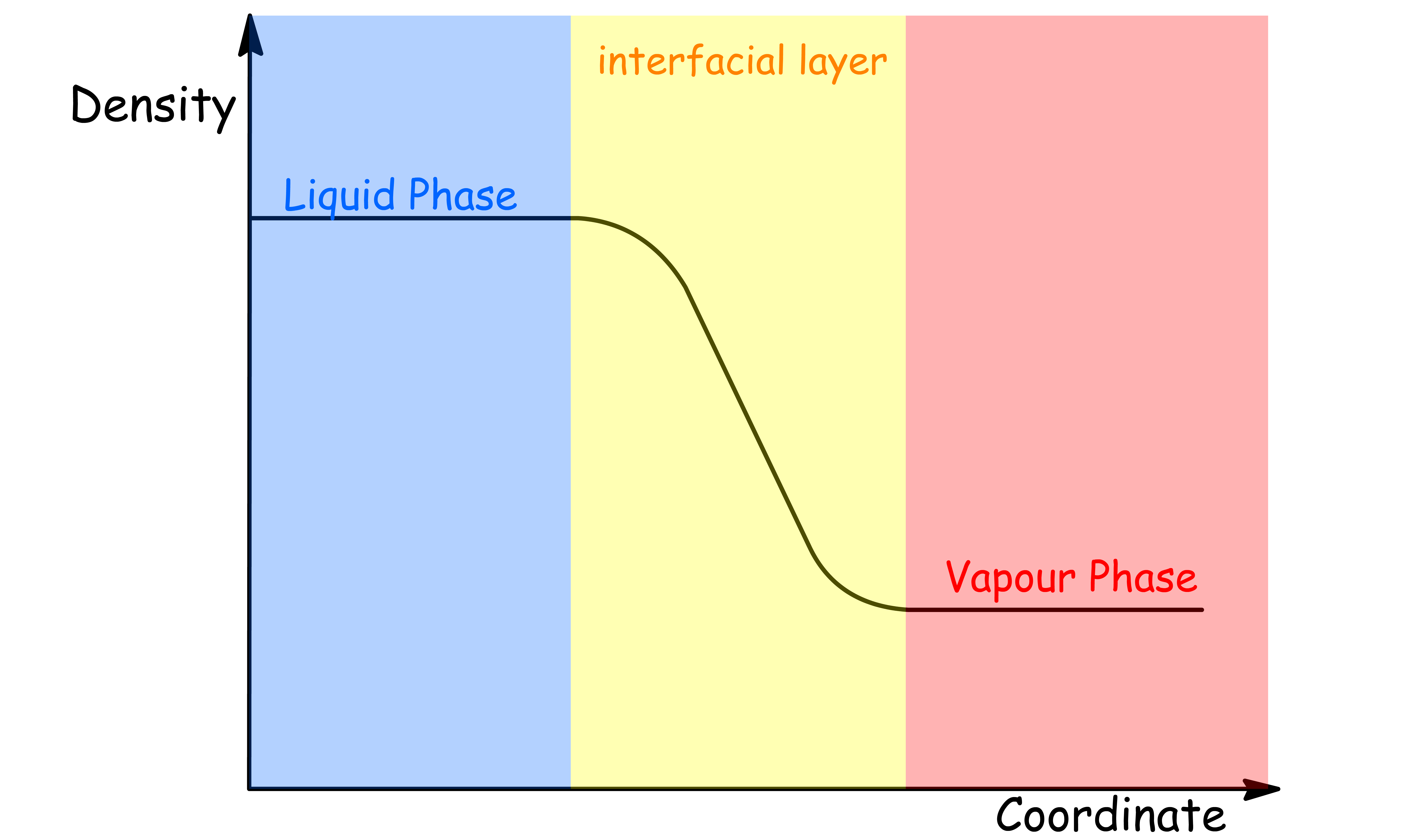
- It provides information on how the density of the molecules changes as a function of distance from the interface
- The system under consideration can consist of either a liquid and a vapor phase, or two liquid phases
We define the location of the interface using the Gibbs Dividing Surface
- This conceptual boundary is chosen to be at a location such that the excess adsorption of a solvent at the interface, denoted as
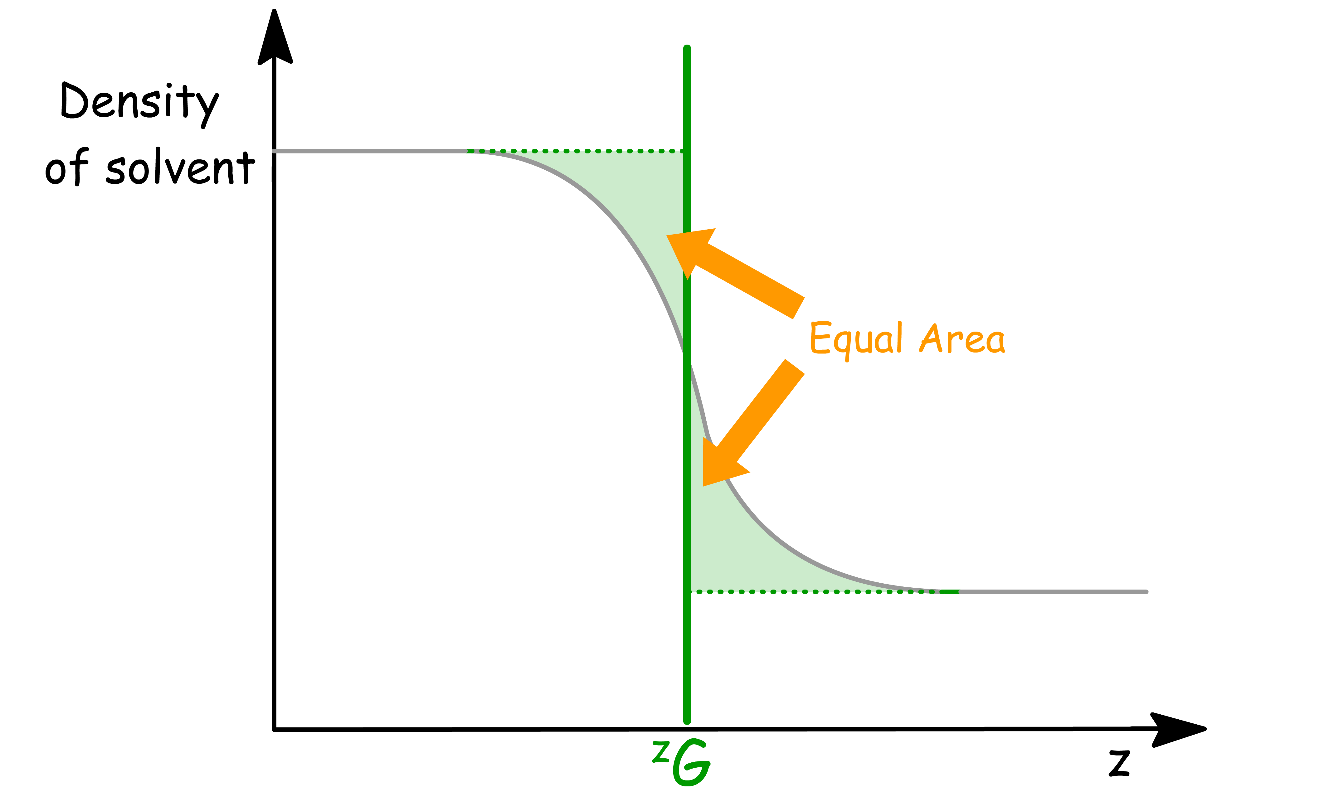
The mass balance condition can be defined mathematically as
- The equation says that the excess mass in the region where the density transitions from to is zero
- In other words, the Gibbs dividing surface is placed such that the total "extra" mass on one side of the surface cancels out the "missing" mass on the other side.
To find the precise location for this dividing surface, we use
- is the gradient of the density across the interface, describing how the density changes with position.
- The integral gives a weighted average of the position , where the weight is the density gradient. This effectively gives the center of mass of the density transition across the interface.
- The factor normalizes this weighted average with respect to the difference in bulk densities of the two phases.
¶ Curved Interfacial Surface
To quantitatively describe curvature of a surface about a point, we shall do the following
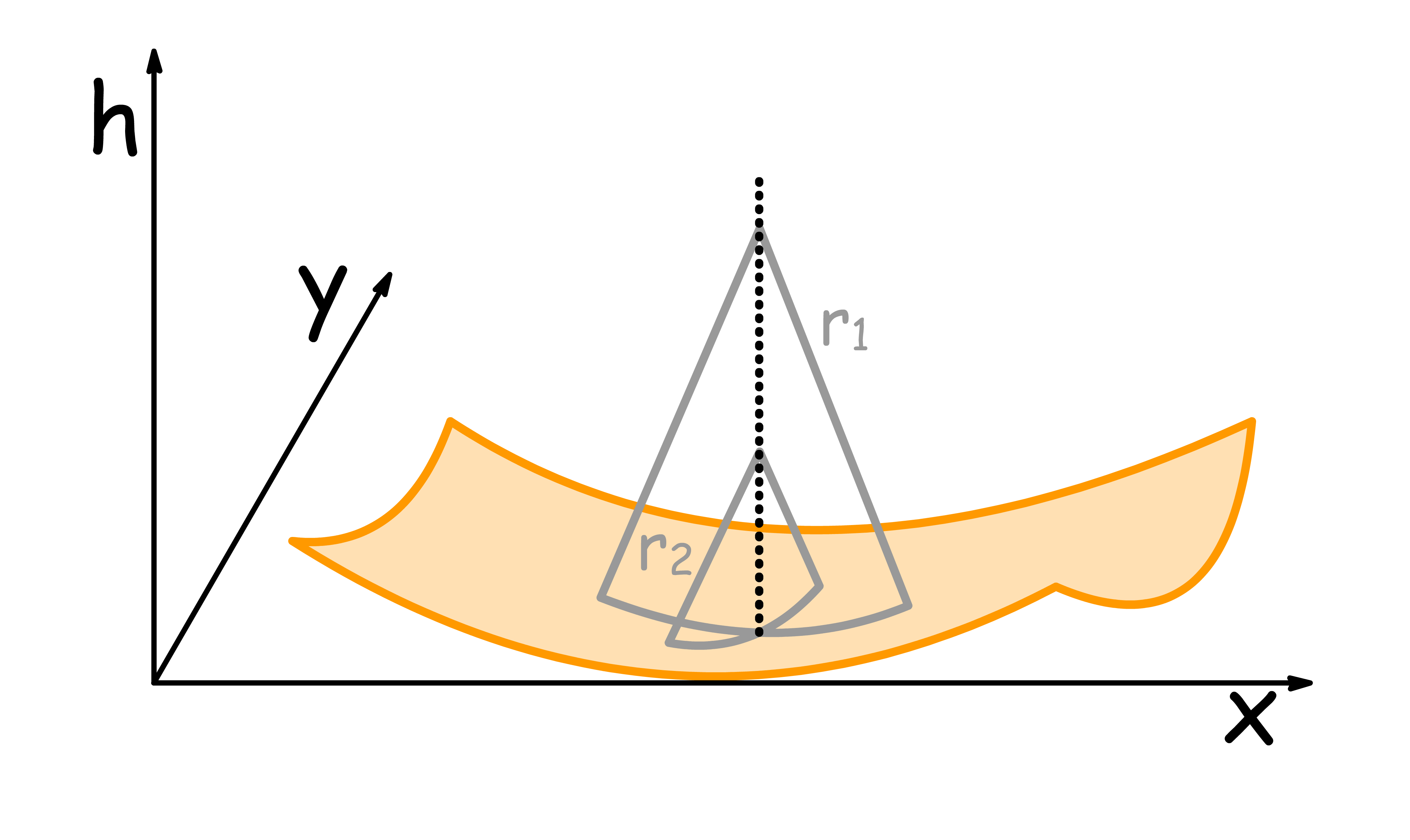
- We draw a line that is normal to the surface of that point
- Randomly draw a circle ( circle 1 ) that has its radius aligned with the line and its perimeter just tangental to the surface
- Draw another circle ( circle 2 ) that also fit the same criteria but is also orthogonal to circle 1
The principle curvatures at that point and are defined as reciprocals of the radii of circle 1 and 2:
To define surface curvatures, we have to define two different curvatures
Mean curvature
It describes how the membrane bends in a local region, averaging the curvatures in orthogonal directions
- For small deviations from a plane, we can approximate it to
- Moreover, the pressure difference across the interface is also dependent on
Gaussian curvature
It measures how the membrane deforms globally, such as whether it twists or forms saddles.
- For small deviations from a plane, we can approximate it to
- The sign of the Gaussian curvature characterises the nature of a surface
Tolman Length
Surface tension is typically considered a constant for flat interfaces, but for curved interfaces, it can vary
- The Tolman equation describes how surface tension depends on the curvature of the interface:
- The Tolman length is a correction factor accounting for curvature, typically in the range of 0.01-0.1 nm
For small droplets or bubbles (on the nanometer scale), this curvature correction becomes significant
- As decreases, the surface tension decreases compared to the planar limit
¶ Capillary Wave Theory
Thermal fluctuations at interfaces cause small undulations, or "waves," that modify the interface's shape and thickness
- These fluctuations are particularly important in systems where surface tension and temperature play major roles in determining the interface's stability
- Capillary Wave Theory (CWT) is a powerful framework used to describe these undulations and predict the behavior of fluctuating interfaces.
The term "capillary waves" refers to undulations on the surface of a fluid that arise due to thermal fluctuations
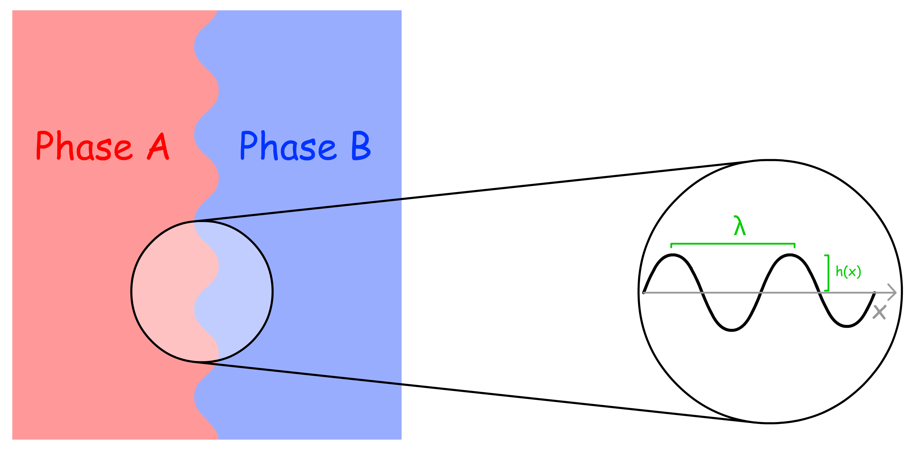
- The wavelength of a capillary wave can vary from molecular scales (nanometers) to millimeters, with larger wavelengths corresponding to lower-energy fluctuations.
- The wavevector is given by q=\frac{2\pi}
- The position of the interface at any horizontal position is denoted as
While a perfectly flat interface might have a sharp boundary, fluctuations smear out this boundary, leading to a finite interfacial thickness.
- The thickness is given by the root mean square :
Spectrum of Capillary Waves
A key feature of CWT is that it predicts a continuous spectrum of waves, each contributing to the overall undulation of the interface.
- The energy associated with each wave depends on its wavelength and surface tension .
- Energy of a fluctuation decreases as the surface tension increases, and also decreases for longer wavelengths.
Free Energy and Capillary Waves
The free energy of an interface is minimized when it remains flat.
- Thermal fluctuations increase the free energy by introducing small deviations from the planar state
For small perturbations from a flat interface, the Hamiltonian (energy function) for capillary waves is given by:
- The free energy due to capillary is given by the difference in surface free energy of the undulated and flat state
Main result of the capillary wave theory
One of the most important results of CWT is that interface thickness increases with the system size
is the mean-square thickness
- When the its value is large,it indicates greater undulations and a thicker, more diffuse interface.
relates the magnitude of the thermal fluctuations to both temperature and surface tension.
- Higher temperatures increase the fluctuations because more thermal energy is available to disturb the interface.
- Higher surface tension dampens the fluctuations, as it acts to resist changes in surface area and restore the interface to its equilibrium state.
The logarithmic factor shows that the mean-square displacement grows as the system size increases relative to the microscopic cutoff length
- is the characteristic length scale of the system (e.g. the lateral size of the interface). The longer the lateral size, the greater the contribution of long-wavelength capillary waves to the overall fluctuations. In large systems, more fluctuations across different scales can occur, leading to a thicker interface.
- is a microscopic cutoff length, often taken as the molecular size or correlation length. It is needed to avoid the equation predicting unphysical behavior at very small scales (). This cutoff represents a lower limit on the length scales over which continuum theories (like Capillary Wave Theory) are valid.
Gravitational Cut-off for Capillary Waves
While the interface thickness theoretically increases without bound with increasing system size, gravity imposes an upper limit on the amplitude of the fluctuations
- This upper limit is governed by the capillary length , which is the length scale beyond which fluctuations are damped by gravitational forces
- (or ) defines the largest wavelength of capillary waves that can be supported by the system before gravity starts to significantly damp them.
- is the density difference between the two phases
Given that gravity imposes an upper limit, we must then modify our previous equation to
- Thus, the largest fluctuations that can exist are of the order of , preventing unbounded growth of the interface thickness.
- This equation accounts for the finite thickness of the interface, limited by gravity and molecular interactions.
¶ Fluctuations of Biological Membranes
Biological membranes are fluid and can deform in response to various forces.
- Membranes are assumed to be in a tensionless state, meaning that there is no external force causing them to stretch or compress.
- To achieve the equilibrium condition (tensionless state), we require that the free energy be at a minimum with respect to changes in the membrane are
Membrane Fluctuations
Membranes fluctuate due to thermal energy. These fluctuations involve undulations and bending of the membrane surface
- Unlike solid surfaces, membranes can undergo bending without significant stretching.
- A parameter for describing of a membrane's resistance to bending is the bending modulus (). A lower value implies the membrane is more flexible.
The Helfrich bending energy model describe the energy cost associated with bending a biological membrane
- The first term, , describes the energy cost due to deviations from the membrane's intrinsic curvature the membrane adopts without any external forces ().
- The second term, , represents the Gaussian curvature energy, which is concerned with the membrane's topological deformations (e.g. how the membrane bends and twists).
Symmetric Membrane and Fourier Transform
The bending energy of a symmetric membrane (with no spontaneous curvature, () is given by
- However, solving this equation directly is complex because of the spatial variations in . To simplify the problem, we express the membrane's thickness function in Fourier space.
In Fourier space, the Laplacian becomes multiplication by , meaning that:
- The bending energy depends on the amplitude of the fluctuations and increases rapidly with the wave vector (because of the term)
- Short-wavelength fluctuations (large ) are much more costly in terms of energy than long-wavelength fluctuations (small ).
Thermal Fluctuations and Equipartition of Energy
Thermal energy causes the membrane to fluctuate, and each wave mode receives a share of the thermal energy due to the equipartition theorem
- According to this principle, each mode contributes:
- The amplitude of the fluctuations decreases with , meaning that large wave vectors (small-wavelength fluctuations) are suppressed by the bending energy
- Larger wavelengths (small ) dominate the fluctuations because they incur a smaller energy cost.
To compute the total mean-square thickness of the membrane, we sum (or integrate) the contributions from all wave modes. This can be done by integrating the mean-square amplitude over all possible wave vectors:
- Hence, the thickness of the membrane grows with the membrane area () and scales inversely with the bending modulus ()
- In other words, larger membranes exhibit more significant overall fluctuations, and stiffer membranes have smaller fluctuations.
Bending Modulus: Flicker Spectroscopy and Simulations
The can be experimentally determined using methods such as flicker spectroscopy
- It measures the spontaneous fluctuations of a membrane in thermal equilibrium
The mean-square displacement of these fluctuations can be related to the bending modulus and the temperature
- Longer-wavelength fluctuations (small ) have larger amplitudes, but are damped by the membrane's bending rigidity.
¶ Wetting and Capillarity
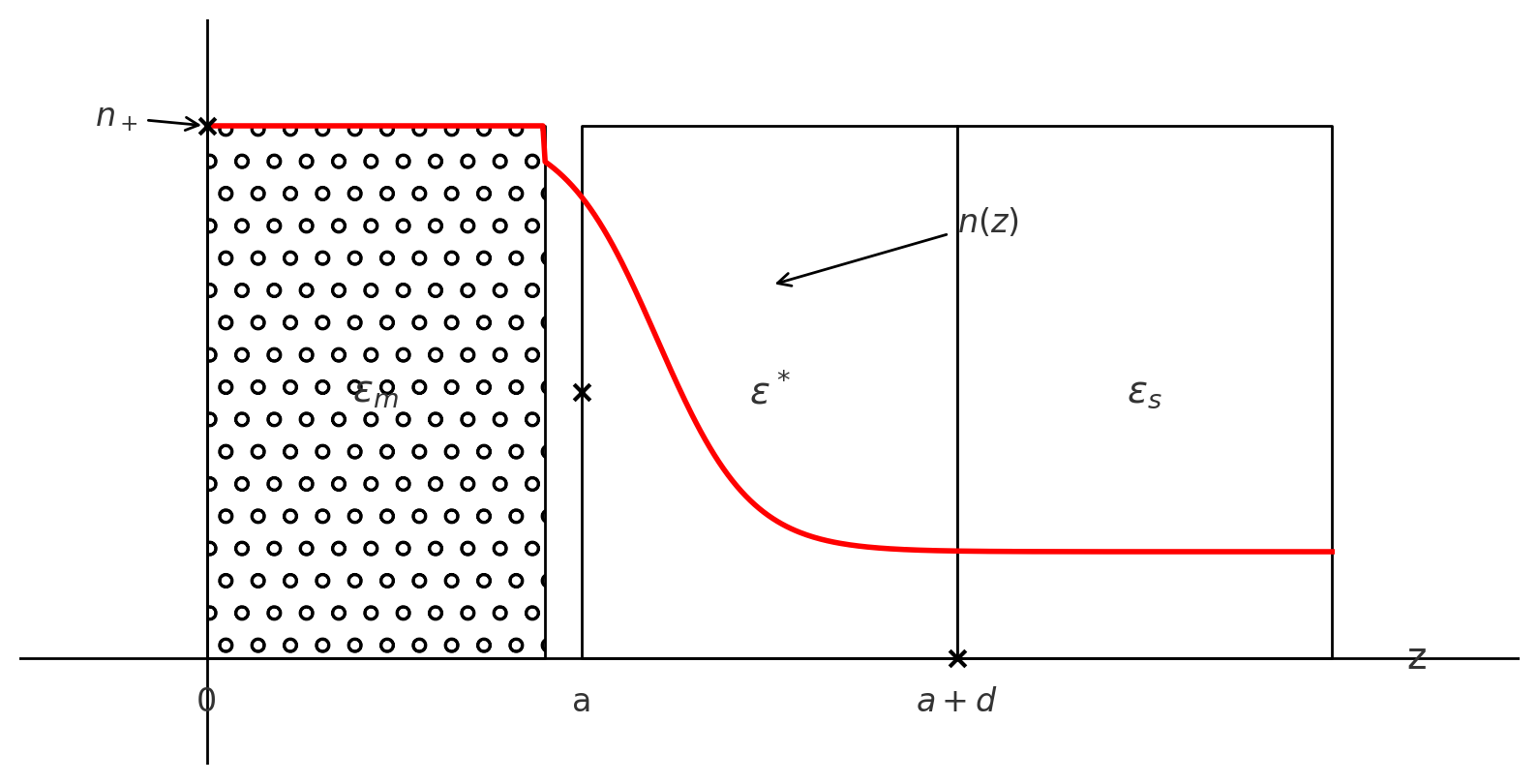
¶ Interface Potential and Wetting Layer Thickness
The interface potential is a function of the wetting layer thickness , where is the thickness of the liquid film on the solid substrate
- The interface potential represents the free energy per unit area required to create and sustain a wetting layer of thickness .
In wetting theory, the wetting layer thickness describes how a liquid spreads over a solid surface
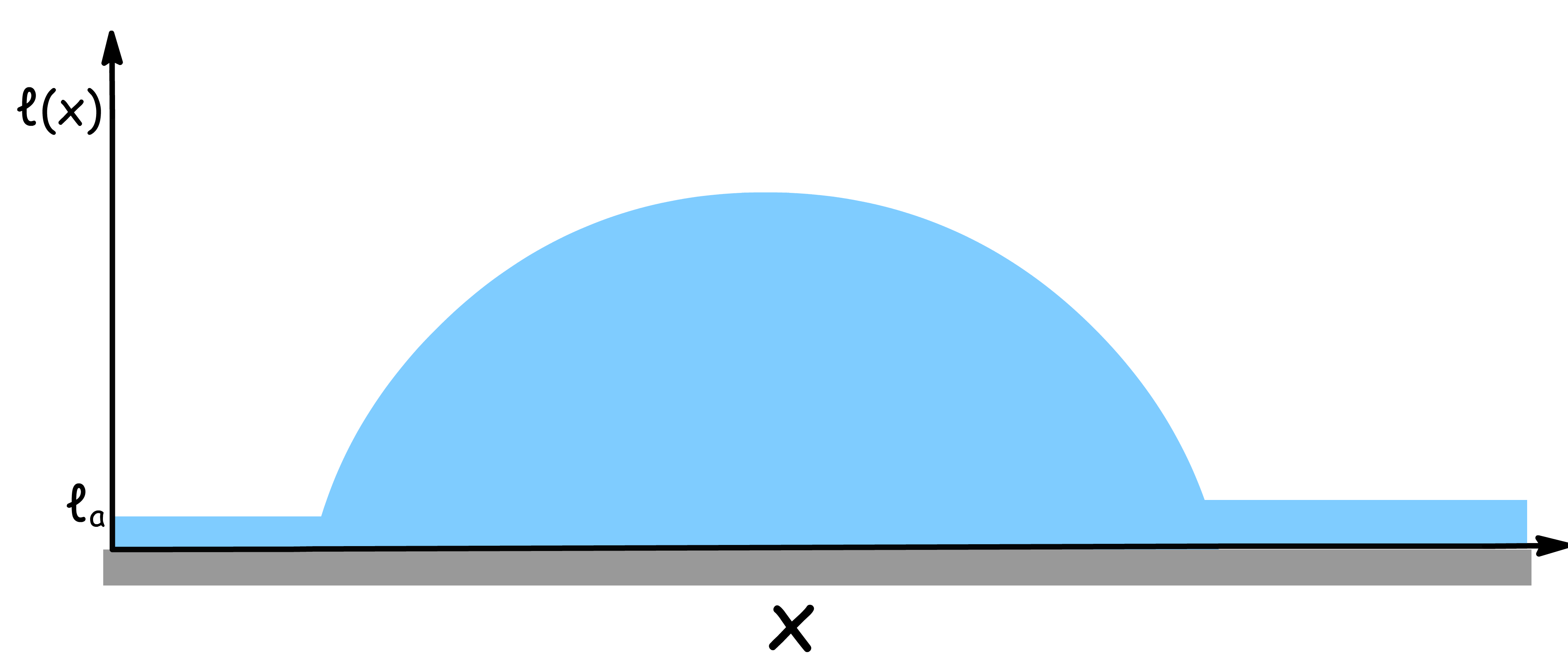
- The film starts with a thin layer, referred to as the precursor film, which has a thickness denoted by the adsorption thickness ( ). The precursor film spreads out uniformly across the surface and is much thinner than the height of the droplet.
- As we move along the surface, increases until it reaches the full droplet thickness.
The interface Potential depends on the relative size of and
- For small deviations of from (i.e. when ), the interface potential can be approximated as:
- For much larger wetting layers (), the interface potential is influenced by several factors, and the approximation becomes:
- This more general expression accounts for various types of forces acting on the wetting layer as its thickness increases
Contributions to the Interface Potential
Van der Waals forces act between the liquid and the substrate. The form of depends on whether the forces are non-retarded (dominant at smaller distances) or retarded (dominant at larger distances):
- Non-retarded van der Waals forces: These are dominant when the wetting layer thickness is small ( ) and can be approximated as:
- Retarded van der Waals forces: For larger thicknesses ( ), retardation effects become important, and the potential decays more rapidly:
- The transition from to occurs due to retardation effects, which weaken the interaction over larger distances as the speed of light influences how these forces propagate.
In systems where electrostatic interactions are present (e.g. ionic liquids, solutions with surface dissociation), Coulombic forces contribute to the interface potential.
- These forces are screened by the presence of dissolved ions, and the screening length ( ) determines how far the electrostatic interactions extend.
- The Coulombic potential is given by:
- Electrostatic forces decay exponentially as the distance increases, with the characteristic length scale determined by the screening effects (e.g., ionic strength in the solution).
¶ Wetting and Pre-Wetting Transitions
The equilibrium wetting layer thickness ( ) corresponds to the point where the system finds mechanical equilibrium for the wetting layer ( i.e. is minimized at that point )
- Since , performing the differentiation will give us
- As , the wetting layer thickness , meaning that the system transitions into a regime of complete wetting where the liquid forms a continuous film on the surface.
The spreading coefficient quantifies the driving force for the liquid to spread across the surface
- If , the liquid completely wets the surface.
- If , the liquid forms droplets on the surface (partial wetting).
- as and
Moreover, wetting transition occurs when
- At this point, the interfacial potential equals the original solid-vapor surface tension, meaning the solid is effectively "replaced" by the liquid, leading to the formation of a thick liquid film on the surface.
The Interfacial Phase Diagram
However, does not increase smoothly as the temperature drop, indicating the existence of phase transitions
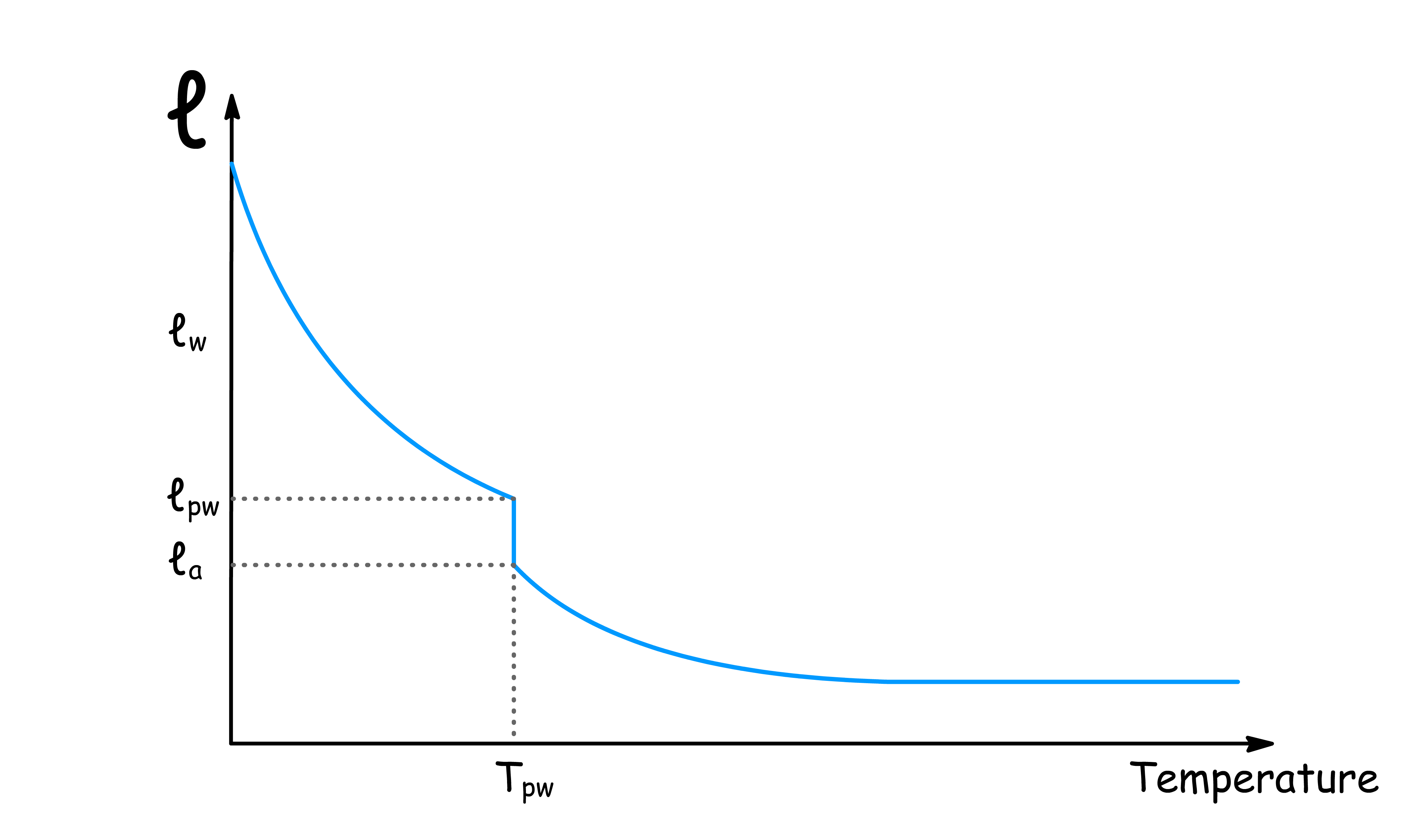
- Complete wetting occurs when the liquid fully coats the surface, and the thickness of the film becomes large, often referred to as
- Prewetting is a first-order phase transition (involves a discontinuous jump in the film thickness) that can occur when the system forms a thin liquid film on the surface, even below the wetting transition temperature
The interfacial phase diagram is a tool used to describe the behavior of surfaces at different temperatures and compositions.
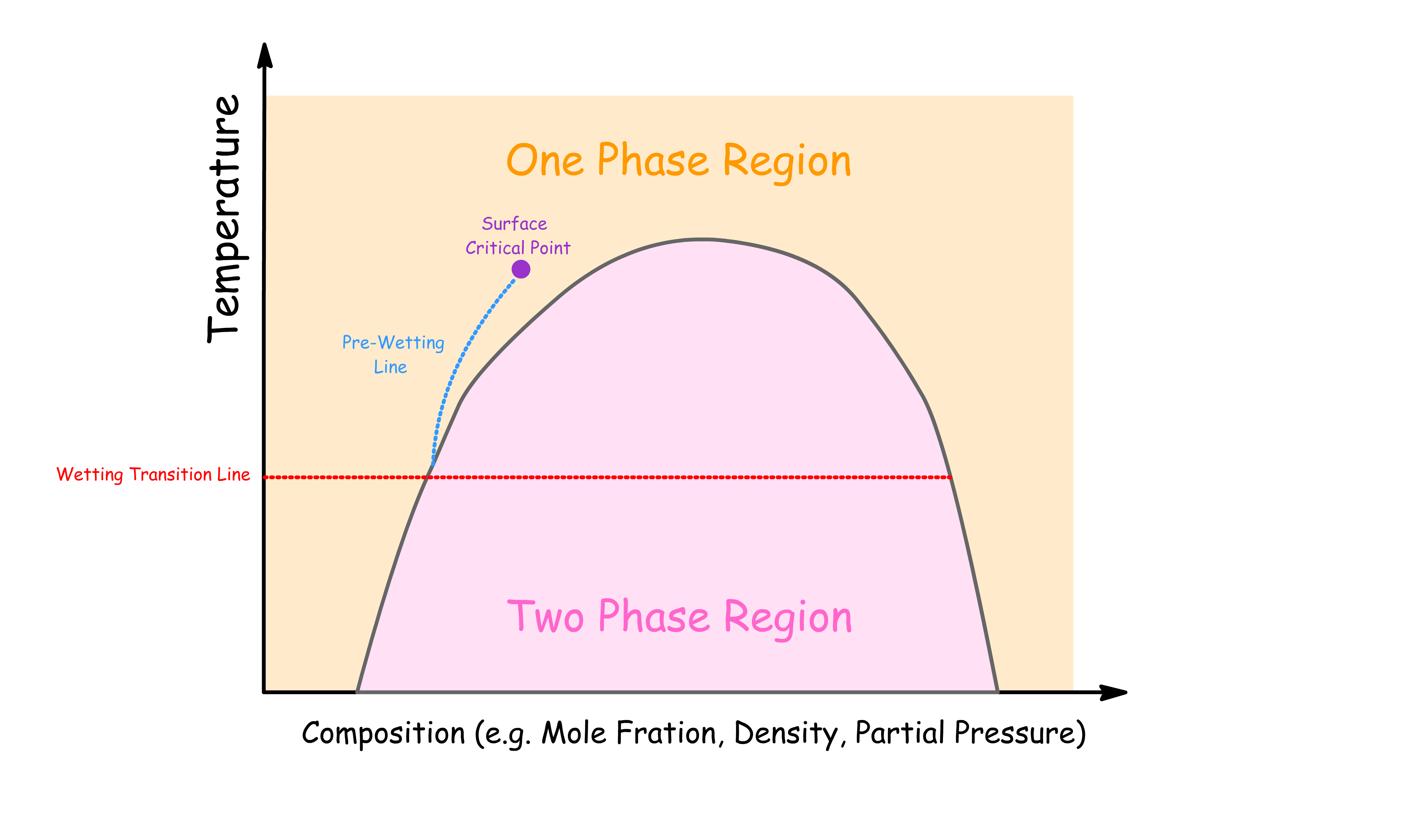
- Prewetting Line: Marks the temperature and chemical potential where a thin film starts to form on the surface. Below this line, the surface is essentially "dry."
- Wetting Transition Line: The temperature where the liquid completely wets the surface, forming a thick or infinite film.
- Surface Critical Point: Where the distinction between phases at the surface vanishes, leading to critical fluctuations in the wetting film.
¶ Three-Phase Line and Line Tension
In the wetting of surfaces, the balance of forces at the three-phase contact line determines the shape and stability of droplets or thin films. These forces include:
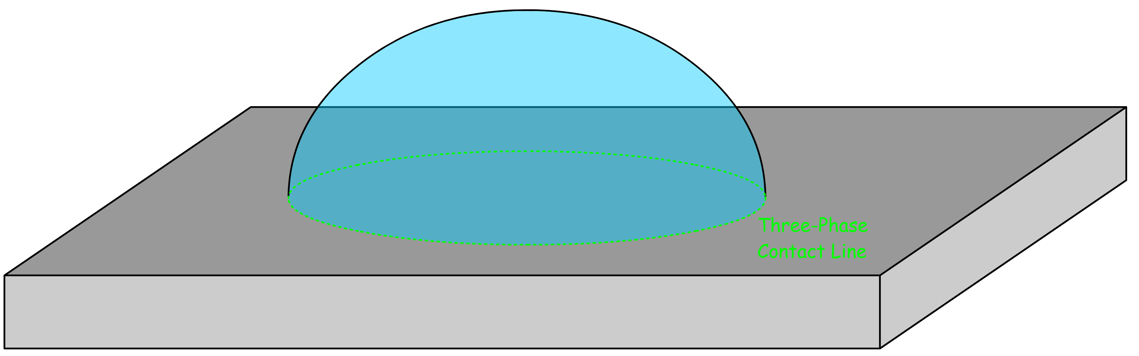
- Surface Tension (): The force acting along the surface of a liquid, which minimizes the surface area.
- Line Tension (): The force acting along the three-phase contact line, contributing to the wetting behavior at very small scales.
Free Energy and Line Tension
The total free energy of the system can be written in differential form, incorporating contributions from temperature (), volume (), chemical potential (), surface area (), and the length of the three-phase contact line ():
- represents the contribution of line tension to the system's free energy, where is the force per unit length along the three-phase contact line.
Line tension length ( ) is a characteristic length scale that relates the line tension ( ) to the surface tension ( ). It provides a measure of how significant line tension effects are compared to surface tension:
- has units of meters (m), and it represents the distance over which line tension significantly affects the wetting behavior.
- When , line tension effects are important.
- For larger droplets, where , the influence of line tension becomes negligible, and surface tension dominates.
The theoretical value of line tension ( ) can be estimated using thermal energy ( ) and a characteristic molecular size ( )
Near Wetting Transitions
Near wetting transitions (when and ), the influence of line tension becomes particularly significant
- The characteristic length scale ( ) associated with line tension near wetting transitions is given by the ratio of the line tension and spreading coefficient:
- As , the approaches the micrometer scale.
- This suggests that as the contact angle decreases (near the point of complete wetting), line tension effects can become important over larger length scales
Contact angle dependence with line tension
The free energy change of the system is given by:
- is the height of the droplet
- is the radius of the droplet's base (contact line radius).
The Young-Laplace equation describes how the contact angle is influenced by surface tensions. However, when line tension is considered, a modified form is used:
- : Three phase line contracts + Doplet beads up
- : Three phase line expands + Doplet spreads out
Temperature plays a role in determining the sign and magnitude of line tension, which in turn affects the contact angle.
- The higher the temperature, the lower the contact angle will be, because positive line tension dominates and contracts the droplet.
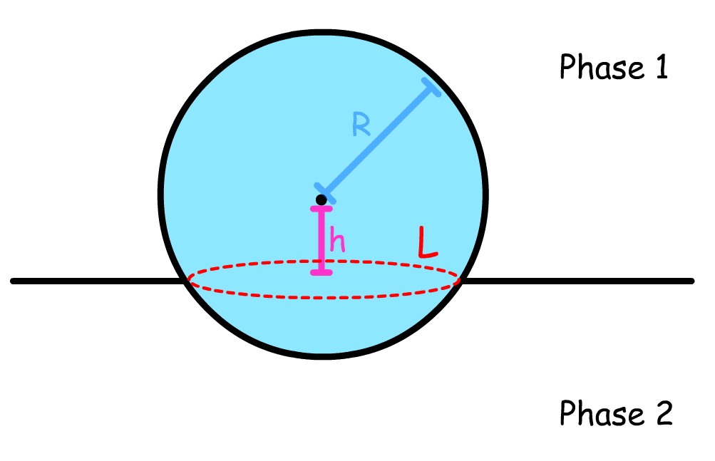
¶ Spherical Particles at Interfaces
The behavior of particles at interfaces depends on their size and the interfacial forces. In particular, the criterion for deformation is given by
- Particles with a radius deform the interface significantly.
The Bond number ( ) determines if deformation can be ignored:
- If , deformation effects are negligible, especially for particles smaller than .
The adsorption behavior of particles at interfaces is size-dependent. The probability of a particle residing at a given height is expressed as:
- Larger particles experience stronger gravitational forces and have lower adsorption probabilities at higher heights due to increased gravitational potential energy.
The interplay of gravitational, thermal, and interfacial forces determines droplets' equilibrium position and distribution.
-
As particle size increases, gravitational forces acting on the particle grow stronger. This causes larger particles to settle downward, while smaller particles are less affected by gravity.
-
Thermal energy counteracts gravitational forces, keeping smaller particles more evenly distributed across the interface.
-
The balance between these two forces sets the particle height ( ) according to the equation:
- Thus, for very small particles (), thermal fluctuations dominate, preventing significant settling.
Thermodynamics
The total free energy for a particle at an interface includes contributions from interfacial tensions and line tension:
- : Interfacial tension between phases 1 and 2.
- : Interfacial tensions between the particle and phases 1 and 2, respectively.
- : Area of the particle in contact with phase 2.
- : Area of the liquid-liquid interface replaced by the particle.
- : Line tension at the three-phase contact line.
- : Length of the three-phase contact line.
The stability of a particle is determined by the derivative of the free energy with respect to the contact angle . For the particle to remain stable, the free energy must exhibit a local minimum.
- The disappearance of the local minimum occurs when the second derivative of the free energy:
- Performing the derivative gives us:
- This expression defines the critical contact angle ( ) at which stability is lost.
The particle is stable at the interface only if its radius exceeds a critical value , given by:
- Smaller particles ( ) are unstable due to the dominating effects of line tension.
- Larger particles ( ) achieve equilibrium as the energy landscape retains a local minimum.
¶ Non-Spherical Particles at Interfaces
The free energy of a non-spherical particle at an interface is given by:
- is the aspect ration and it is given by
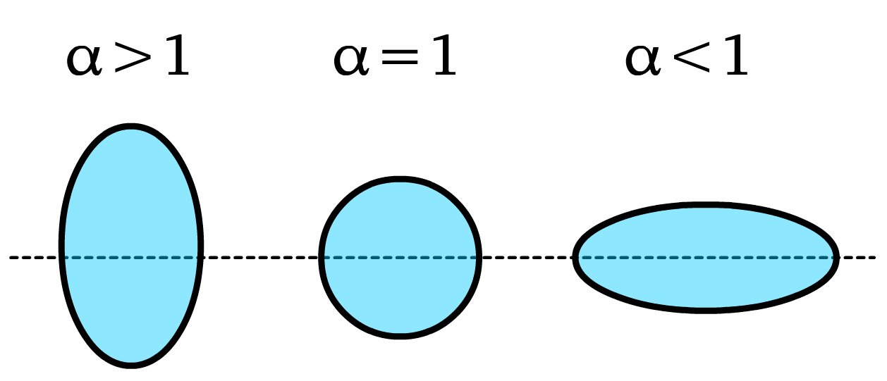
Anisotropy and Interfacial Deformations
- Monopolar Deformation ():
- For particles with significant gravitational effects or external fields, large interfacial distortions dominate.
- Dipolar Deformation:
- Observed under external torque or applied fields.
- Causes particles to rotate and align asymmetrically.
- Quadrupolar Deformation:
- Intrinsic to anisotropic particles.
- Occurs even without external forces and is governed by the Young-Laplace equation:
- Deformations depend on both aspect ratio () and the contact angle, where larger have stronger quadrupolar effects and smaller have weaker deformations.
¶ Electrochemical Interfaces
Electrochemical interfaces involve the interaction between a conductive electrode and an electrolyte, where the redistribution of charges at the interface results in phenomena such as capacitance, adsorption, and electrochemical reactions.
¶ Capacitance
Capacitance at these interfaces plays a central role in describing charge storage and dynamic response.
The electrode is modeled as an equivalent circuit consisting of:
- A capacitance ( ), representing charge storage at the interface.
- A resistance ( ), representing Faradaic processes or charge transfer resistance.
The total impedance ( ) of the system is given by:
- In order for the measurement to be accurate, the capacitive contribution dominates:
Differential and Integral Capacitance
Capacitance at electrochemical interfaces can be described in terms of differential and integral capacitance:
Differential Capacitance ( ) :
- Measures the rate of change of charge with respect to the applied potential
- Differential capacitance is typically determined experimentally by measuring the charge response to small changes in potential.
Integral Capacitance ( ):
- Integral capacitance is typically calculated and provides a broader measure of charge storage over a potential range, integrating both adsorption and structural effects.
The relationship between and captures how the local capacitance changes with potential:
- The term represents the contribution from total stored charge, while accounts for variations in storage behavior as potential changes.
- When changes slowly with potential, . But rapid variations in lead to significant differences between and .
Electrocapillary Phenomena
Electrocapillary phenomena describe how surface tension ( ) at an electrode-electrolyte interface is influenced by surface charge ( ) and applied potential ( ).
The basic equation of electrocapillarity links changes in surface tension to surface charge and the chemical potential ( ) of adsorbing species:
- If the solution composition remains constant ( ), the equation simplifies to the Lippmann Equation:
- This provides a direct relationship between surface charge and the slope of the electrocapillary curve:
The electrocapillary curve exhibits the following features:
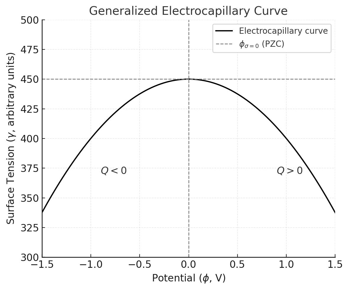
- Parabolic Shape: The curve peaks at the potential of zero charge ( ), where and .
- Charge Dependence:
- For : Positive charge accumulates ().
- For : Negative charge dominates ().
Capacitance can also be derived from the second derivative of surface tension with respect to potential:
- Differential capacitance quantifies the local response of surface tension to changes in potential.
- Peaks in occur at points of rapid surface charge redistribution.
The surface tension of a stationary liquid drop is influenced by gravitational and geometric factors.
The instantaneous current is proportional to the surface charge density and the rate of surface expansion ( ):
The averaged current over a drop period is:
- : Maximum surface area during drop formation.
Helmholtz Layer and Capacitance
The Helmholtz layer describes the compact, immobile layer of ions at an electrode-electrolyte interface
- The electric field ( ) across the Helmholtz layer is proportional to the surface charge density ( $sigma$ ):
- The potential drop ( ) across the Helmholtz layer is related to the field and the thickness of the layer ( ):
- From this relationship, the surface charge density can be expressed as:
Surface tension at the interface varies with potential () according to the Lippmann equation:
- Integrating this relationship gives the total surface tension as:
- This leads to the inverted parabolic shape of the electrocapillary curve, where surface tension reaches a maximum at the potential of zero charge .
The differential capacitance of the Helmholtz layer, which quantifies its ability to store charge, is derived from the relationship between charge and potential:
- Substituting () into this expression will give us the capacitance of the Helmholtz layer!!!
Base on this relationship, we can understand a few important things
- Charge Separation: The Helmholtz layer acts like a parallel plate capacitor, with ions on the electrolyte side and electrons/holes on the electrode side.
- Electrocapillary Behavior: The parabolic dependence of surface tension on potential highlights the balance between charge density and potential drop.
- Capacitance: Helmholtz capacitance is independent of the ionic concentration in the solution, as it only depends on and .
¶ Gouy-Chapman Theory
The Gouy-Chapman theory provides allows us to understand the diffuse electrical double layer formed at the interface of a charged electrode and electrolyte.
Fundamental Assumptions
The theory is built upon the Poisson-Boltzmann approximation and assumes:
- The energy of an ion is determined only by the electric field and screened by the solvent.
- No fluctuations or chemical interactions between ions and the solvent.
The potential profile across the interface is governed by the Poisson Equation:
- The potential gradient at the interface:
Surface Charge Density
The surface charge density is given by:
- is a scaling factor related to ion concentration and Debye length and is given by
- is the Bjerrum Length represents the scale of electrostatic interactions
For a 1:1 electrolyte:
Capacitance of the Double Layer
The capacitance ( ) of the electrochemical interface is determined by the effective screening length ( )
- is the modified Debye length, which accounts for the influence of surface potential ( ) and is defined as:
- is the normy Debye length, representing the intrinsic screening length and relates to the Bjerrum Length () and the bulk ionic concentration ( )
Using the hyperbolic cosine identity and the expression for surface charge, the effective length ( ) can be rewritten in terms of ( ):
If we define and , we can rewrite in a simpler manner because why not
The Electrocappilary Equation
The surface tension is related to the surface potential () as:
- At higher electrolyte concentrations, the surface tension varies significantly with potential.
- The curves flatten as the electrolyte concentration decreases, consistent with reduced ionic screening.
Potential Profiles
The Gouy-Chapman theory describes the electric potential and charge distribution in the electrical double layer formed at the interface between an electrode and electrolyte.
As mentioned before, the dimensionless potential is defined as:
Dimensionless distance, is expressed in terms of the Debye length
The potential profile accounts for both non-linearized and linearized scenarios:
- Non-linearized Potential Profile:
Accounts for large values of , with exponential decay modified by ionic correlations.
- This exact form considers the influence of stronger potentials.
- Linearized Approximation (Weak Potentials):
Suitable for weak potentials where the ionic distribution is approximately symmetric.
- When , the potential simplifies to:
- This describes a simple exponential decay.
The charge distribution in the double layer is governed by:
- This equation captures the density of ions near the charged electrode.
¶ Graham Theory
Graham theory is critical for understanding interfacial capacitance in systems where no specific ionic adsorption occurs. It combines the contributions of different capacitances, enabling the characterization of interfacial phenomena.
The surface charge density () is:
- A negative indicates the charge's role in balancing the counter-ions in the diffuse layer.
The potential difference at the interface is split into components:
By defining the total interfacial capacitance () as the inverse of , the total capacitance () can be expressed as:
- Helmholtz Capacitance (): Represents the contribution from the compact layer directly adjacent to the electrode. It does not depend on electrolyte concentration, but can depend on the charge
- Diffuse Capacitance (): Captures the influence of the Gouy-Chapman diffuse layer. Use the equation derived earlier
Hence, the slowest (smallest) capacitance dominates the total response, making it easier to identify the limiting factor in the system.
The Parsons-Zobel plot represents the relationship between the inverse of total capacitance and the inverse of the diffuse layer capacitance
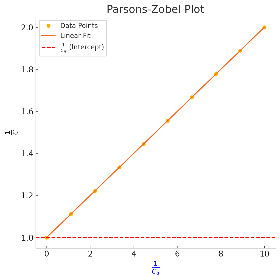
- The y-intercept is the reciprocal of the Helmholtz layer capacitance. This is significant as remains independent of the bulk ionic concentration.
¶ Mean Field Molecular Models of the Compact Layer
¶ Two-States
The mean field molecular model aims to describe the electrostatic and thermodynamic behavior of a charged compact layer, such as that observed in ionic or electronic systems.
- This model provides insights into the distribution of particles (e.g. electrons, ions) and the resulting electric field, capacitance, and polarization under applied potentials.
- By simplifying the complex interactions within the layer to a "two-state" system, the model focuses on the competition between up () and down () states of particles and their alignment with the applied electric field.
Assumptions
Two-State Model
The two-state model assumes particles in the system can exist in only two discrete energy states, labeled up () and down ().
- These states may correspond to physical orientations (dipole alignment in an electric field)
Mean Field Approximation
This approximation used to simplify many-body problems. In this context, rather than accounting for the detailed interactions between individual particles, the effect of all particles is averaged into a single, uniform field.
- This significantly reduces computational complexity while retaining key macroscopic behaviors, especially for systems with large particle numbers where fluctuations around the mean are small.
- It is particularly effective in studying systems like compact layers, where the field primarily depends on the net charge distribution.
The energy of each state is influenced by the applied electric field , and the population of these states depends on the Boltzmann distribution:
The order parameter, , quantifies the alignment of particles with the field:
- is the total particle density
- is the critical potential and is defined as:
- The potential satisfies the self-consistent relation:
Two-State Capacitance
The surface charge density, , is expressed as:
The differential (Helmholtz) capacitance, , measures the sensitivity of surface charge to changes in potential:
- is the intrinsic (geometric) capacitance
- is the effective screening length
¶ Fawcett Three-State Model
The model introduces a third state () to account for molecules that are neither completely aligned nor anti-aligned with the field.
- This additional state helps reproduce the Helmholtz capacitance for aprotic solvents by fitting the residual energies of these three states.
- This model is particularly suited for systems where non-uniform orientations dominate under weak fields.
Frumkin-Damaskin-Parsons Cluster Model
The cluster model extends the molecular description by incorporating clustering effects, where molecules form groups with lower residual energy.
- Clusters minimize energy and dominate in zero electric fields due to low residual energy.
- In strong fields, clusters disband into individual molecules, leading to higher dipole moments.
Particle Distribution:
The total population is distributed among:
- Individual Molecule Populations:
- Cluster Molecule Populations:
- is the effective dipole moment of a cluster.
serves as a normalization factor and is given by
- The electric field satisfy closure: E = \frac{4\pi \sigma}{\varepsilon_\infty} = \frac{\phi}
The key assumption is that molecules in clusters have no preferential dipole orientation within the cluster, as .
The potential difference is influenced by both individual and clustered molecules:
The differential capacitance incorporates contributions from both molecule populations:
¶ Metal Contribution to Double Layer Capacitance
Our overlord ✨Kornyshev✨ have cited his own paper on equations that describe contribution of metallic electrons to capacitance in double-layer systems. The model incorporates both spatial charge distribution effects and dielectric properties to refine the classical Helmholtz picture.
The Helmholtz capacitance, ( ), is expressed as:
- : Closest distance of approach of excess charge to the metal surface.
- : Center of mass of the excess charge distribution:
- : Effective dielectric thickness of the layer.
- : Dielectric constant as a function of the surface charge density ().
This equation highlights the competition between , which is fixed by physical constraints, and , which is determined by the spatial distribution of charge.
The differential capacitance, ( ), includes dynamic factors:
- : Modified center of mass for differential charge, dependent on ().
- : Sensitivity of to changes in surface charge density, accounting for ionic rearrangements.
- : Effective dielectric constant that incorporates charge density effects.
The two type of capacitance are related by
¶ Surface Electronic Profiles
The surface electronic density, ( ), describes the deviation from the neutral state and is defined as:
- : Electronic profile influenced by the field.
- : Neutral density.
This equation ensures charge conservation, connecting the surface charge ( ) with the electronic density profile. It forms the foundation for calculating the total energy ( ).
The energy functional ( ) captures the contributions of electrostatics, quantum mechanics, and surface interactions:
- : Hartree energy from electrostatic interactions.
- : Kinetic energy of the electronic profile.
- : Exchange-correlation energy, describing electron interactions.
- : Pseudopotential energy due to interaction with the surface.
Trial Function Approach
To simplify the calculation, ( ) is approximated using a trial function:
- : Mean position of the electronic profile.
- : Scaling function, describing decay.
This trial function connects the profile ( ) to physical parameters such as , providing a basis for energy calculations.
- Total energy functional:
- Center of mass of the excess charge:
Simplifying:
The center of mass ( ) measures the average spatial position of the excess charge ( ) relative to the surface.
- : Actual charge density profile in the presence of surface charge ( ).
- : Neutral charge density profile, serving as the reference.
This equation builds on the trial function approach, where is explicitly modeled to describe the spatial distribution of electrons. Using the trial function’s symmetry and decay properties, simplifies to:
- represents the mean position of charge, derived from the trial function.
- : The decay parameter, describing how rapidly diminishes spatially.
¶ Something about water
Gradient Expansion and Short-Range Forces
The first theoretical approach by Marčelja and Radić (1976) described water using an order parameter profile , where:
- This expansion leads to exponentially decaying forces due to water’s correlation lengths. The derivative of the free energy functional gives pressure as:
indicating exponentially decaying structural forces within short ranges.
Field Theory in Pure Water
In field theory, three fields are introduced:
(electric field), (displacement field), (polarization density field).
The Hamiltonian is decomposed into electrostatic and water correlation contributions:
The correlation function and dielectric function link these fields, yielding three correlation lengths:
- : exponential decay lengths
- : oscillation wavelength.
Coupled Differential Equations for Water Correlations
Minimizing the functional between two surfaces gives:
- relates to oscillatory (overscreening) correlations, and to Lorentzian (exponential) correlations
- Bulk water behavior is established within $\sim$1 nm of the surface.
Force Calculations and Solvation Phenomena
The total force is derived from the Hamiltonian:
- \Pi_{tot} = \Pi_{dir, DLVO} + \Pi_
- Solvation oscillations trap ions in deep “water wells” and overscreening occurs at higher concentrations.
¶ Ising Theory of Order-Disorder Transitions
The Ising model is applied to describe order-disorder transitions in adsorbed ionic or molecular layers at an electrode. It models interactions between nearest-neighbor adsorption sites using the Hamiltonian:
- : represents the adsorption states.
- : Coupling constants for horizontal and vertical nearest-neighbor interactions.
These transitions occur between two specific configurations of adsorbed particles:
1. Ordered Phase
- Phase
- Adsorbed particles occupy every site uniformly.
2. Different Ordered Phase
- Phase
- The phase involves alternating adsorption rows
Using these, the coupling constants ( ) and ( ) can be expressed in terms of the observed energy difference, :
The critical temperature () dictates when these transitions occur between ordered and disordered phases.
Relating the coupling constants () to . This in turns allows to connect and :
- For , the phase boundary can be written out with a linear approximation:
- This approximation is used to construct the - phase diagram:
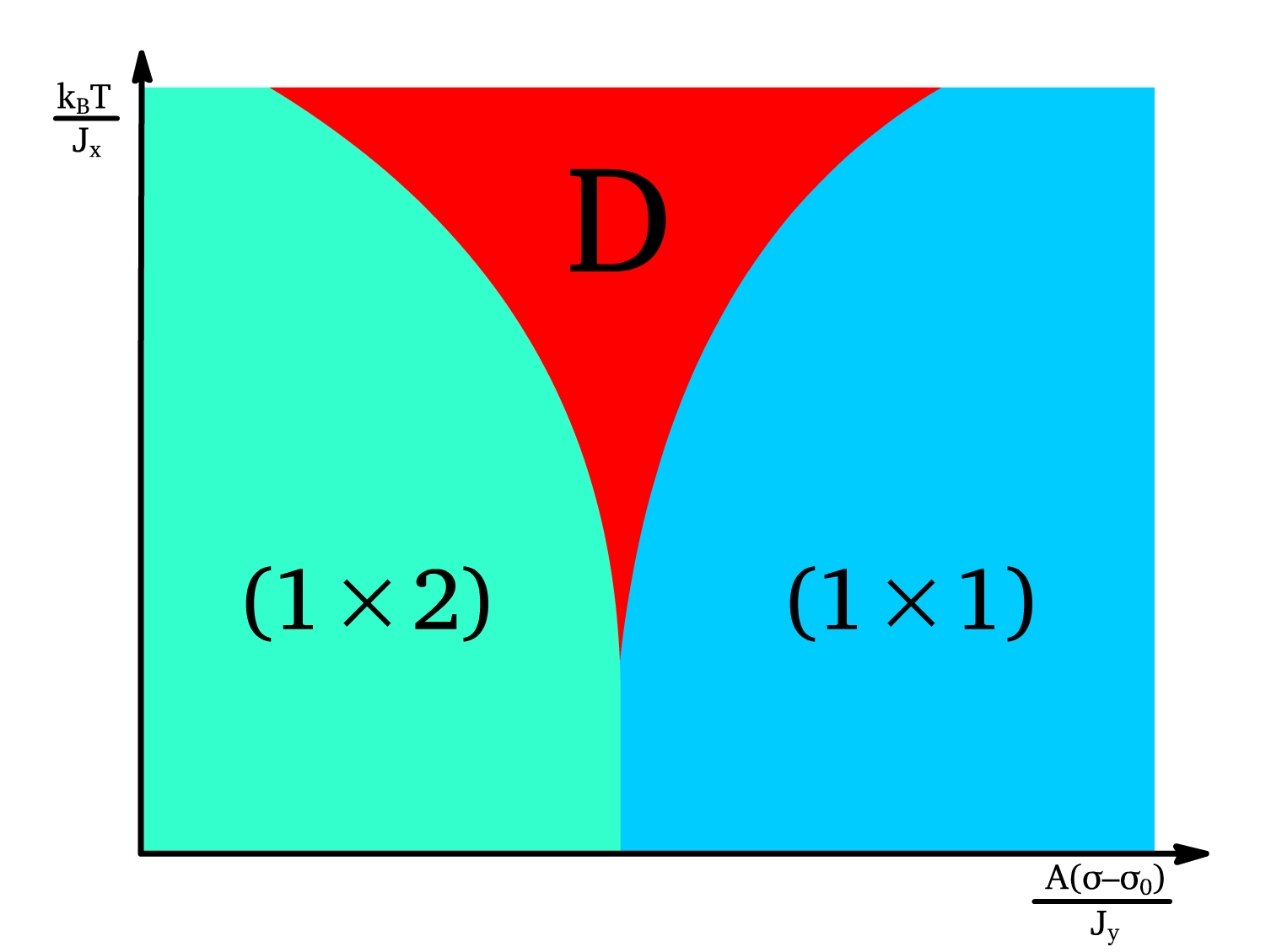
Disordered Region:
The ( ) and ( ) phases are separated by a disordered region ( ), where neither phase dominates.
- The width of the disorder region is:
¶ Ising Order Parameter
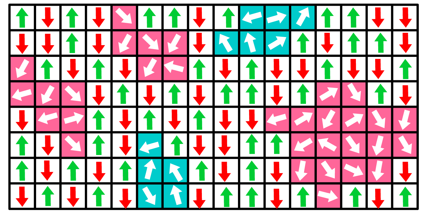
The Ising order parameter is a quantitative measure of the surface reconstruction state. It distinguishes between reconstructed and unreconstructed configurations of the surface and is defined as:
- and represent the dimensions of the lattice.
- is a spin-like variable denoting the state of the surface atoms. Positive and negative values of correspond to different surface orientations or configurations.
The value of tells us what state the system is in
1. Reconstructed State
- Fully reconstructed surface with ordered domains
2. Unreconstructed State
- Represents the absence of reconstruction, where surface atoms are randomly or uniformly distributed without domain formation.
exhibits critical behavior near the reconstruction transition and scales with the reduced temperature ( ) or reduced charge ( ):
Here:
- : Critical temperature at which reconstruction occurs.
- : Critical charge density.
- : Critical exponent for the Ising model.
Roughening and Ising Lines in the Free Fermion Theory
The roughening transition of steps on a surface can be understood through the partition function of a single step that occasionally jumps between neighboring atomic rows
The free energy associated with the step is . Setting , the roughening temperature is derived:
For domain walls on an Ising surface, a similar expression describes the Ising transition temperature
The step energy for reconstructed and unreconstructed surfaces depends on their configuration:
- Energy of the lowest step of unreconstructed surface ():
- Energy of the lowest step of reconstructed surface ():
The energy of an Ising wall relates to the () step energy:
Kink energies on domain walls and steps are connected:
Full Phase Diagram
The roughening of the unreconstructed () state involves the formation of () steps, which destabilize the surface. The associated charge () is given by:
- is the reference energy for kink formation, and relates to the surface charge per area.
- Higher temperatures promote step roughening by overcoming the energy barrier .
Conversely, the roughening of the reconstructed () state occurs through the introduction of () steps. The charge () for this transition is expressed as:
- Compared to the () roughening, this transition involves a stronger dependence on temperature due to the coefficient , emphasizing the greater energy required to disrupt the reconstructed state.
As the temperature increases further, the surface transitions from ordered to disordered configurations.
- This transition involves breaking the long-range order in reconstructed domains, with the charge given by:
- Here, the smaller energy barrier compared to roughening transitions indicates that the order-disorder transition is less energetically demanding.
By combining these transitions, the phase diagram is constructed with distinct boundaries corresponding to the roughening and Ising transitions.
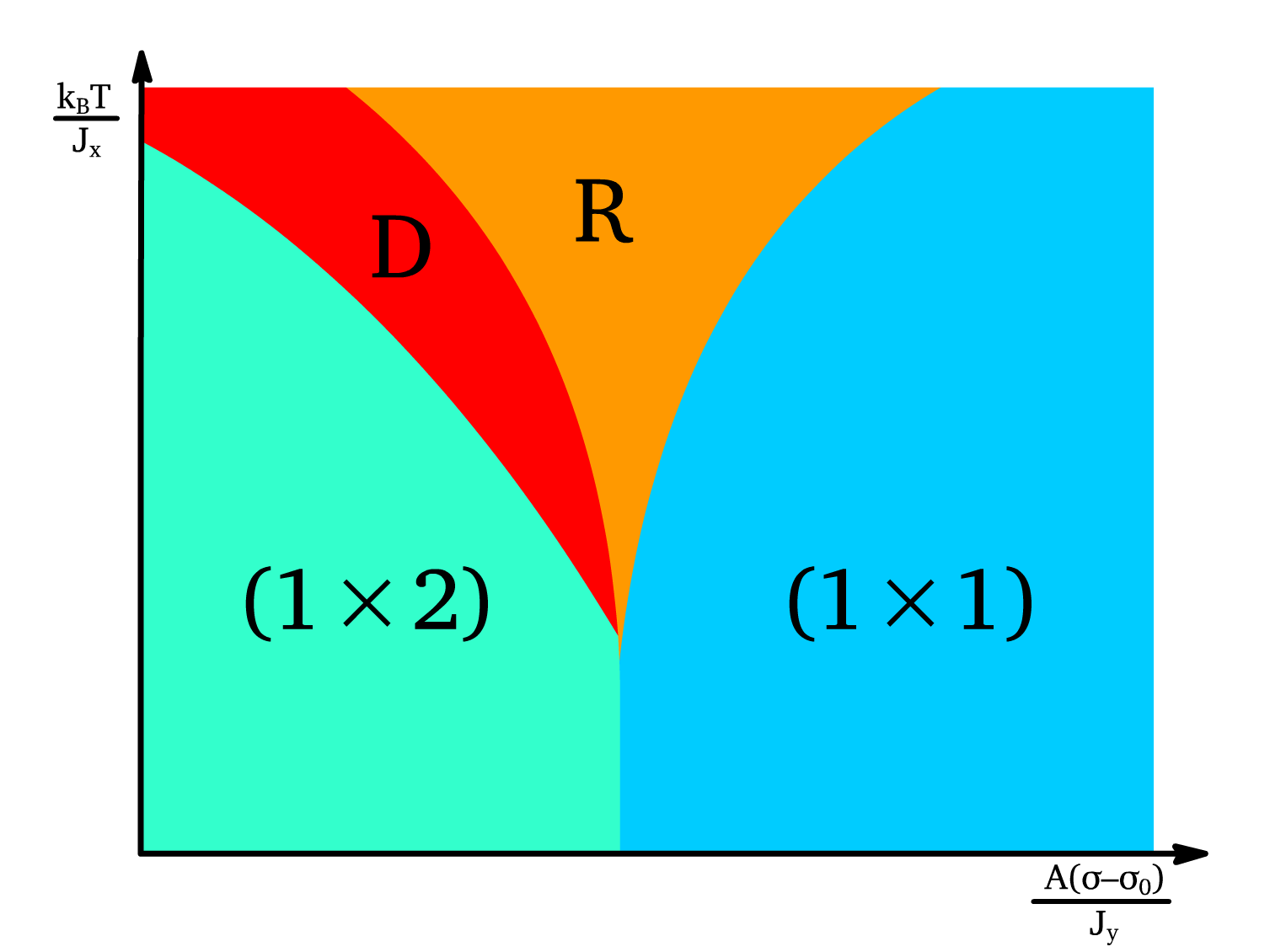
- The roughening transitions () and () define the limits of stability for the () and () states, while () marks the transition to a disordered state.
- The relationships ensure consistency between the step kink energies and domain wall energies
¶ Ionic Liquid
Lattice Gas Model and Ionic Distributions in Bulk and at Interfaces
We can use a lattice gas model to describe ionic liquids by quantifying ionic distributions in bulk and at interfaces under an electric potential. The free energy functional, , forms the core of this model. It is given by:
- and are the numbers of cations and anions, respectively, is the total number of available sites
- is the electric potential.
Minimizing the free energy functional with respect to and yields the equilibrium ion distributions, and .
A central parameter , defined as , represents the ratio of total ions in the bulk to total available sites
- ties bulk concentration () to the maximum possible ionic concentration ().
The distribution configurations for ions and holes are captured via the partition terms:
- The total configurational term is , and its logarithm simplifies via Stirling’s formula:
Neglecting higher-order interactions such as and simplifies the chemical potentials:
- In the bulk (), , where is the average density.
The behavior of ionic distributions near an electrode under the influence of an electric potential is captured using Fermi-like distributions.
- When , these equations reduce to the Boltzmann distributions.
The electrostatic potential distribution follows the Poisson-Fermi equation:
For , this simplifies to the Gouy-Chapman equation.
Capacitance at the Electrode-Ionic Liquid Interface
The mean-field capacitance of an ionic liquid interface is influenced by and , where is the Debye capacitance.
- The general expression for capacitance is:
- For the incompressible liquid case (), this reduces to:
Camel and Bell Shaped Capacitance Curves
The dependence of on leads to characteristic shapes:
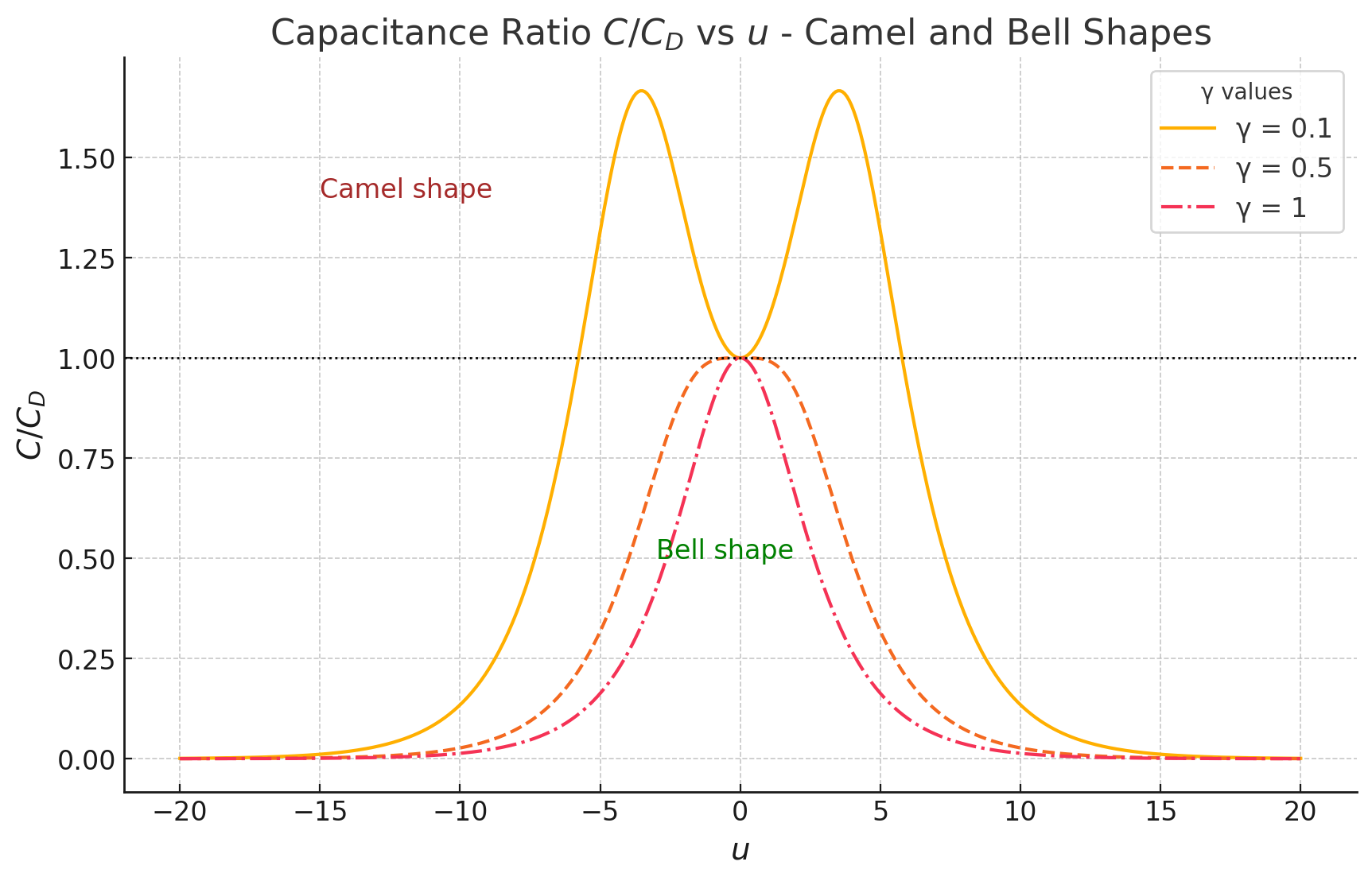
- Camel Shape: Observed at moderate values where capacitance peaks for both positive and negative potentials.
- Bell Shape: At low , capacitance peaks symmetrically around zero potential.
For small potentials () and (the demarcation point), the capacitance approximately follows:
Lattice Saturation Branches and Weak Temperature Dependence of Capacitance
The capacitance at the lattice saturation branches of ionic systems shows a weak or negligible dependence on temperature.
- : Dimensionless potential scaled by thermal energy.
- : Maximum ionic concentration in the lattice.
- : Ratio of bulk ion concentration to the saturation concentration.
Capacitance Behavior at Lattice Saturation and Phenomenological Asymmetry
For , where the system approaches lattice saturation:
- and L_\text{eff} \approx L_D \sqrt
The lattice saturation law simplifies:
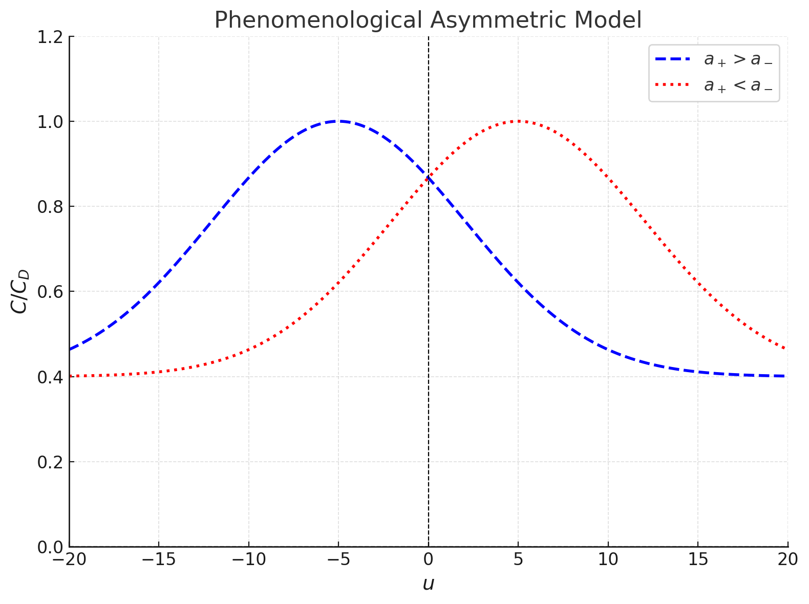
The free energy functional, , describes the system under an external potential :
- and are the numbers of cations and anions.
- and are parameters reflecting ionic interaction effects.
The differential capacitance is derived from the free energy:
- is the reduced potential.
- is the normalized capacitance factor: .
- is the asymmetry parameter: with and representing ionic properties and the ionic saturation factor.
The graph below presents as a function of , showing dependence on :
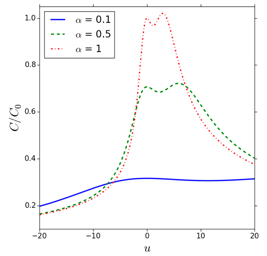
- As increases in value, the symmetry increases
Diffusion and Kinetics of Ionic Exchange
The diffusion coefficient is temperature-dependent and follows the Arrhenius equation:
The modified Nernst-Einstein relation incorporates ion-specific properties, expressed as:
- : Concentration,
- : Ion probabilities,
The survival probability function determines the state dynamics of ions:
- represents the state of a molecule:
The lifetime of an ion is calculated as:
Kinetics of Exchange Process:
- Free and Bound States: The survival probability function is studied for both free and bound states of ions.
- Exponential Models: The data are fitted using exponential and biexponential decay models:
where and represent fast and slow time constants.
Two-State System with Exchange Theory: Velocity Autocorrelation Function (VACF)
The two-state exchange model describes molecular motion in systems where ions or molecules transition between free and bound states. The dynamics are captured using the Velocity Autocorrelation Function (VACF), denoted as :
- : Probability of the free state.
- : Probability of the bound state.
The probability that a molecule remains in the same state over time is given by:
- : Fraction of ions in fast relaxation,
- : Fast relaxation time,
- : Slow relaxation time.
The derivative of , , describes the decay rate of the survival probability.
The VACF is expressed in the -domain (Laplace transform) as:
- : Laplace transform of ,
- : Laplace transform of .
The VACF in the time domain is reconstructed as:
where the overall VACF is a weighted sum of the contributions from free and bound states.
Anomalous Capacitance
The anomalous capacitance phenomenon in conducting nanopores is explained using the concept of a "superionic state". In slit nanopores, the electrostatic potential is described by:
- is the radial distance, the slit width, and the Bjerrum length in confinement
- This demonstrates the periodicity and decay of electrostatic interactions within nanopores.
The energy stored in a capacitor is expressed as:
Two-State Model with Nearest-Neighbor Interactions in Ionophilic Pores:
The two-state model describes the nearest neighbor interactions within ionophilic pores. The Hamiltonian is expressed as:
- represents the charge state of site , with possible values of or .
- quantifies the interaction strength between nearest neighbors.
- , combining the potential difference and the energy associated with ion transfer to the pore interior.
The ionic charge density per unit surface area of the pore is:
- is the total number of sites, and is the pore perimeter
The capacitance per unit surface area is:
- being the Bjerrum length in vacuum.
The interaction potential between charges of the same or opposite signs at a distance is:
- is the pore radius,
- is the Bjerrum length, with for ionic liquids.